limit%20forms%20as%20%E2%84%91%CF%84%E2%86%920%2B

SearchAdvancedHelp

(0.010 seconds)

11—20 of 837 matching pages

11: 27.2 Functions

… ►where $p_1,p_2,\mathrm{\dots },p_{\nu \left(n\right)}$ are the distinct prime factors of $n$, each exponent $a_r$ is positive, and $\nu \left(n\right)$ is the number of distinct primes dividing $n$. …Euclid’s Elements (Euclid (1908, Book IX, Proposition 20)) gives an elegant proof that there are infinitely many primes. … ►An equivalent form states that the $n$th prime $p_n$ (when the primes are listed in increasing order) is asymptotic to $n\ln n$ as $n\to \mathrm{\infty }$: … ►The $\varphi \left(n\right)$ numbers $a,a^2,\mathrm{\dots },a^{\varphi \left(n\right)}$ are relatively prime to $n$ and distinct (mod $n$). …It is the special case $k=2$ of the function $d_k\left(n\right)$ that counts the number of ways of expressing $n$ as the product of $k$ factors, with the order of factors taken into account. …

12: 8.26 Tables

… ►

Khamis (1965) tabulates $P(a,x)$ for $a=0.05(.05)10(.1)20(.25)70$, $0.0001\le x\le 250$ to 10D.

… ►

Abramowitz and Stegun (1964, pp. 245–248) tabulates $E_n\left(x\right)$ for $n=2,3,4,10,20$, $x=0(.01)2$ to 7D; also $(x+n){\mathrm{e}}^x{E}_n\left(x\right)$ for $n=2,3,4,10,20$, $x^{-1}=0(.01)0.1(.05)0.5$ to 6S.

►

Chiccoli et al. (1988) presents a short table of $E_p\left(x\right)$ for $p=-\frac{9}{2}(1)-\frac{1}{2}$, $0\le x\le 200$ to 14S.

►

Pagurova (1961) tabulates $E_n\left(x\right)$ for $n=0(1)20$, $x=0(.01)2(.1)10$ to 4-9S; ${\mathrm{e}}^x{E}_n\left(x\right)$ for $n=2(1)10$, $x=10(.1)20$ to 7D; ${\mathrm{e}}^x{E}_p\left(x\right)$ for $p=0(.1)1$, $x=0.01(.01)7(.05)12(.1)20$ to 7S or 7D.

… ►

Zhang and Jin (1996, Table 19.1) tabulates $E_n\left(x\right)$ for $n=1,2,3,5,10,15,20$, $x=0(.1)1,1.5,2,3,5,10,20,30,50,100$ to 7D or 8S.

13: 18.40 Methods of Computation

… ►Orthogonal polynomials can be computed from their explicit polynomial form by Horner’s scheme (§1.11(i)). … ►It is now necessary to take the limit $\epsilon \to 0+$ of $F(x^{\prime }+\mathrm{i}\epsilon )$, and the imaginary part is the required Stieltjes–Perron inversion: …Results of low ($2$ to $3$ decimal digits) precision for $w(x)$ are easily obtained for $N\sim 10$ to $20$. Gautschi (2004, p. 119–120) has explored the $\epsilon \to 0^{+}$ limit via the Wynn $\epsilon$-algorithm, (3.9.11) to accelerate convergence, finding four to eight digits of precision in $w(x)$, depending smoothly on $x^{\prime }$, for $N\approx 4000$, for an example involving first numerator Legendre OP’s. … ►Convergence is $\sim O\left(N^{-2}\right)$. …

14: 8 Incomplete Gamma and Related
Functions

…

15: 28 Mathieu Functions and Hill’s Equation

…

16: Bibliography R

… ►

Normal limit theorems for symmetric random matrices. Probab. Theory Related Fields 112 (3), pp. 411–423.

ⓘ

External Links:

ISSN 0178-8051, Document, MathReview (Alexei Khorunzhy), ZentralBlatt

Referenced by:

§35.9.

Encodings:

BibTeX

… ►

On the definition and properties of generalized $6$-$j$ symbols. J. Math. Phys. 20 (12), pp. 2398–2415.

ⓘ

External Links:

ISSN 0022-2488, Document, MathReview (S. Saran), ZentralBlatt

Referenced by:

§16.4(iii), §16.4(iii).

Encodings:

BibTeX

… ►

Uniform asymptotic approximations to the solutions of the Orr-Sommerfeld equation. I. Plane Couette flow. Studies in Appl. Math. 53, pp. 91–110.

ⓘ

External Links:

MathReview (T. W. Kao), ZentralBlatt

Referenced by:

§2.8(iii).

Encodings:

BibTeX

… ►

Applied Bessel Functions. Dover Publications Inc., New York.

ⓘ

Notes:

Reprint of original Blackie & Son Limited, London, 1946.

External Links:

MathReview, ZentralBlatt

Referenced by:

§10.73(iii).

Encodings:

BibTeX

… ►

On Simple Waves with Profiles in the form of some Special Functions—Chebyshev-Hermite, Mathieu, Whittaker—in Two-phase Media. In Differential Operators and Related Topics, Vol. I (Odessa, 1997), Operator Theory: Advances and Applications, Vol. 117, pp. 313–322.

ⓘ

External Links:

ISBN 3-7643-6287-1, MathReview Entry, ZentralBlatt

Referenced by:

5th item.

Encodings:

BibTeX

…

17: 4.31 Special Values and Limits

§4.31 Special Values and Limits

►

Table 4.31.1: Hyperbolic functions: values at multiples of $\frac{1}{2}\pi \mathrm{i}$.

► ►►

$z$	0	$\frac{1}{2}\pi \mathrm{i}$	$\pi \mathrm{i}$	$\frac{3}{2}\pi \mathrm{i}$	$\mathrm{\infty }$
…

►

►

4.31.1 $$\underset{z\to 0}{lim}\frac{\sinh z}{z}=1,$$

ⓘ

Symbols:

$\sinh z$: hyperbolic sine function and $z$: complex variable

Permalink:

http://dlmf.nist.gov/4.31.E1

Encodings:

pMML, png, TeX

See also:

Annotations for §4.31 and Ch.4

►

4.31.2 $$\underset{z\to 0}{lim}\frac{\tanh z}{z}=1,$$

ⓘ

Symbols:

$\tanh z$: hyperbolic tangent function and $z$: complex variable

Permalink:

http://dlmf.nist.gov/4.31.E2

Encodings:

pMML, png, TeX

See also:

Annotations for §4.31 and Ch.4

►

4.31.3 $$\underset{z\to 0}{lim}\frac{\cosh z-1}{z^2}=\frac{1}{2}.$$

ⓘ

Symbols:

$\cosh z$: hyperbolic cosine function and $z$: complex variable

Permalink:

http://dlmf.nist.gov/4.31.E3

Encodings:

pMML, png, TeX

See also:

Annotations for §4.31 and Ch.4

18: 1.12 Continued Fractions

… ► $A_n$ and $B_n$ are called the $n$th (canonical) numerator and denominator respectively. … ►A contraction of a continued fraction $C$ is a continued fraction $C^{\prime }$ whose convergents $\{C_n^{\prime }\}$ form a subsequence of the convergents $\{C_n\}$ of $C$. …The even part of $C$ exists iff $b_{2k}\ne 0$, $k=1,2,\mathrm{\dots }$, and up to equivalence is given by … ►A continued fraction converges if the convergents $C_n$ tend to a finite limit as $n\to \mathrm{\infty }$. … ►The continued fraction ${\displaystyle \frac{a_1}{b_1+}\frac{a_2}{b_2+}\mathrm{\cdots }}$ converges when …

19: 22.3 Graphics

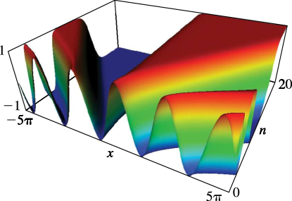
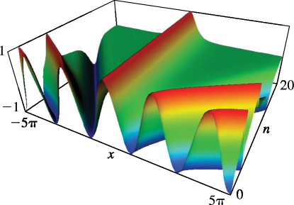
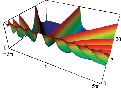
… ►Line graphs of the functions $\mathrm{sn}(x,k)$, $\mathrm{cn}(x,k)$, $\mathrm{dn}(x,k)$, $\mathrm{cd}(x,k)$, $\mathrm{sd}(x,k)$, $\mathrm{nd}(x,k)$, $\mathrm{dc}(x,k)$, $\mathrm{nc}(x,k)$, $\mathrm{sc}(x,k)$, $\mathrm{ns}(x,k)$, $\mathrm{ds}(x,k)$, and $\mathrm{cs}(x,k)$ for representative values of real $x$ and real $k$ illustrating the near trigonometric ($k=0$), and near hyperbolic ($k=1$) limits. … ►

►

►

Figure 22.3.13: $\mathrm{sn}(x,k)$ for $k=1-{\mathrm{e}}^{-n}$, $n=0$ to 20, $-5\pi \le x\le 5\pi$. Magnify 3D Help

►

►

►

Figure 22.3.14: $\mathrm{cn}(x,k)$ for $k=1-{\mathrm{e}}^{-n}$, $n=0$ to 20, $-5\pi \le x\le 5\pi$. Magnify 3D Help

►

►

►

Figure 22.3.15: $\mathrm{dn}(x,k)$ for $k=1-{\mathrm{e}}^{-n}$, $n=0$ to 20, $-5\pi \le x\le 5\pi$. Magnify 3D Help

… ►

►►

Figure 22.3.28: Density plot of $|\mathrm{sn}(20,k)|$ as a function of complex $k^2$, $-10\le \mathrm{\Re }\left(k^2\right)\le 20$, $-10\le \mathrm{\Im }\left(k^2\right)\le 10$. … Magnify

…

20: 33.24 Tables

… ►

Abramowitz and Stegun (1964, Chapter 14) tabulates $F_0(\eta ,\rho )$, $G_0(\eta ,\rho )$, $F_0^{\prime }(\eta ,\rho )$, and $G_0^{\prime }(\eta ,\rho )$ for $\eta =0.5(.5)20$ and $\rho =1(1)20$, 5S; $C_0\left(\eta \right)$ for $\eta =0(.05)3$, 6S.

►

Curtis (1964a) tabulates $P_{\mathrm{\ell }}(ϵ,r)$, $Q_{\mathrm{\ell }}(ϵ,r)$ (§33.1), and related functions for $\mathrm{\ell }=0,1,2$ and $ϵ=-2(.2)2$, with $x=0(.1)4$ for and $x=0(.1)10$ for $ϵ\ge 0$; 6D.

…