fold%20canonical%20integral

SearchAdvancedHelp

(0.002 seconds)

11—20 of 475 matching pages

11: 36.4 Bifurcation Sets

… ► $K=1$, fold bifurcation set: … ►

$x=\frac{9}{20}{z}^2.$

… ►

$x=-\frac{3}{20}{z}^2,$

…

12: 19.2 Definitions

… ►

§19.2(i) General Elliptic Integrals

… ►is called an elliptic integral. … ►

§19.2(ii) Legendre’s Integrals

… ►

§19.2(iii) Bulirsch’s Integrals

… ►

§19.2(iv) A Related Function: $R_C(x,y)$

…

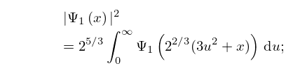
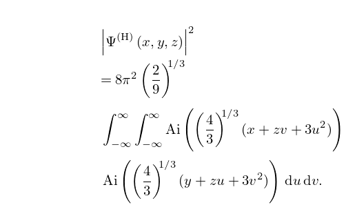
13: 36.9 Integral Identities

§36.9 Integral Identities

►

36.9.1 $${|{\mathrm{\Psi }}_1\left(x\right)|}^2=2^{5/3}{\int }_0^{\mathrm{\infty }}{\mathrm{\Psi }}_1\left(2^{2/3}(3u^2+x)\right)du;$$

ⓘ

Symbols:

${\mathrm{\Psi }}_K\left(𝐱\right)$: canonical integral function, $dx$: differential of $x$ , $\int$: integral and $x$: real parameter

Permalink:

http://dlmf.nist.gov/36.9.E1

Encodings:

pMML, png, TeX

See also:

Annotations for §36.9 and Ch.36

… ►

36.9.8 $${\left|{\mathrm{\Psi }}^{(\mathrm{H})}\left(x,y,z\right)\right|}^2=8{\pi }^2{\left(\frac{2}{9}\right)}^{1/3}{\int }_{-\mathrm{\infty }}^{\mathrm{\infty }}{\int }_{-\mathrm{\infty }}^{\mathrm{\infty }}\mathrm{Ai}\left({\left(\frac{4}{3}\right)}^{1/3}(x+zv+3u^2)\right)\mathrm{Ai}\left({\left(\frac{4}{3}\right)}^{1/3}(y+zu+3v^2)\right)dudv.$$

ⓘ

Symbols:

$\mathrm{Ai}\left(z\right)$: Airy function, $\pi$: the ratio of the circumference of a circle to its diameter, $dx$: differential of $x$ , ${\mathrm{\Psi }}^{(\mathrm{H})}\left(𝐱\right)$: hyperbolic umbilic canonical integral function, $\int$: integral, $y$: real parameter, $z$: real parameter and $x$: real parameter

Permalink:

http://dlmf.nist.gov/36.9.E8

Encodings:

pMML, png, TeX

See also:

Annotations for §36.9 and Ch.36

… ►For these results and also integrals over doubly-infinite intervals see Berry and Wright (1980). …

14: 36.6 Scaling Relations

§36.6 Scaling Relations

… ►

${\mathrm{\Psi }}_K(𝐱;k)=k^{{\beta }_K}{\mathrm{\Psi }}_K\left(𝐲(k)\right),$

►

${\mathrm{\Psi }}^{(\mathrm{U})}(𝐱;k)=k^{{\beta }^{(\mathrm{U})}}{\mathrm{\Psi }}^{(\mathrm{U})}\left({𝐲}^{(\mathrm{U})}(k)\right),$

… ►

Indices for $k$-Scaling of Magnitude of ${\mathrm{\Psi }}_K$ or ${\mathrm{\Psi }}^{(\mathrm{U})}$ (Singularity Index)

… ►

Table 36.6.1: Special cases of scaling exponents for cuspoids.

► ►►►

singularity	$K$	${\beta }_K$	${\gamma }_{1K}$	${\gamma }_{2K}$	${\gamma }_{3K}$	${\gamma }_K$
fold	1	$\frac{1}{6}$	$\frac{2}{3}$	$-$	$-$	$\frac{2}{3}$
…

►

…

15: 20 Theta Functions

Chapter 20 Theta Functions

…

16: 21.8 Abelian Functions

… ►An Abelian function is a $2g$-fold periodic, meromorphic function of $g$ complex variables. …

17: 36.3 Visualizations of Canonical Integrals

§36.3 Visualizations of Canonical Integrals

►

§36.3(i) Canonical Integrals: Modulus

… ►

§36.3(ii) Canonical Integrals: Phase

►In Figure 36.3.13(a) points of confluence of phase contours are zeros of ${\mathrm{\Psi }}_2\left(x,y\right)$; similarly for other contour plots in this subsection. In Figure 36.3.13(b) points of confluence of all colors are zeros of ${\mathrm{\Psi }}_2\left(x,y\right)$; similarly for other density plots in this subsection. …

18: 36.5 Stokes Sets

… ►

§36.5(ii) Cuspoids

… ►

36.5.7 $$X=\frac{9}{20}+20u^4-\frac{Y^2}{20u^2}+6u^2\mathrm{sign}\left(z\right),$$

ⓘ

Symbols:

$\mathrm{sign}x$: sign of, $z$: real parameter, $X$: scaled coordinate and $Y$: scaled coordinate

Permalink:

http://dlmf.nist.gov/36.5.E7

Encodings:

pMML, png, TeX

See also:

Annotations for §36.5(ii), §36.5(ii), §36.5 and Ch.36

… ►

§36.5(iii) Umbilics

… ►

§36.5(iv) Visualizations

… ►Red and blue numbers in each region correspond, respectively, to the numbers of real and complex critical points that contribute to the asymptotics of the canonical integral away from the bifurcation sets. …

19: 8.26 Tables

… ►

Khamis (1965) tabulates $P(a,x)$ for $a=0.05(.05)10(.1)20(.25)70$, $0.0001\le x\le 250$ to 10D.

… ►

§8.26(iv) Generalized Exponential Integral

►

Abramowitz and Stegun (1964, pp. 245–248) tabulates $E_n\left(x\right)$ for $n=2,3,4,10,20$, $x=0(.01)2$ to 7D; also $(x+n){\mathrm{e}}^x{E}_n\left(x\right)$ for $n=2,3,4,10,20$, $x^{-1}=0(.01)0.1(.05)0.5$ to 6S.

… ►

Pagurova (1961) tabulates $E_n\left(x\right)$ for $n=0(1)20$, $x=0(.01)2(.1)10$ to 4-9S; ${\mathrm{e}}^x{E}_n\left(x\right)$ for $n=2(1)10$, $x=10(.1)20$ to 7D; ${\mathrm{e}}^x{E}_p\left(x\right)$ for $p=0(.1)1$, $x=0.01(.01)7(.05)12(.1)20$ to 7S or 7D.

… ►

Zhang and Jin (1996, Table 19.1) tabulates $E_n\left(x\right)$ for $n=1,2,3,5,10,15,20$, $x=0(.1)1,1.5,2,3,5,10,20,30,50,100$ to 7D or 8S.

20: 36 Integrals with Coalescing Saddles

Chapter 36 Integrals with Coalescing Saddles

…