elliptic integrals

SearchAdvancedHelp

(0.014 seconds)

31—40 of 132 matching pages

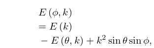
31: 19.11 Addition Theorems

§19.11 Addition Theorems

… ►

19.11.7 $$F(\varphi ,k)=K\left(k\right)-F(\theta ,k),$$

ⓘ

Symbols:

$K\left(k\right)$: Legendre’s complete elliptic integral of the first kind, $F(\varphi ,k)$: Legendre’s incomplete elliptic integral of the first kind, $\varphi$: real or complex argument, $k$: real or complex modulus and $\theta$: amplitude

Permalink:

http://dlmf.nist.gov/19.11.E7

Encodings:

pMML, png, TeX

See also:

Annotations for §19.11(ii), §19.11 and Ch.19

►

19.11.8 $$E(\varphi ,k)=E\left(k\right)-E(\theta ,k)+k^2\sin \theta \sin \varphi ,$$

ⓘ

Symbols:

$E\left(k\right)$: Legendre’s complete elliptic integral of the second kind, $E(\varphi ,k)$: Legendre’s incomplete elliptic integral of the second kind, $\sin z$: sine function, $\varphi$: real or complex argument, $k$: real or complex modulus and $\theta$: amplitude

Permalink:

http://dlmf.nist.gov/19.11.E8

Encodings:

pMML, png, TeX

See also:

Annotations for §19.11(ii), §19.11 and Ch.19

… ►

§19.11(iii) Duplication Formulas

… ►

19.11.12 $$F(\psi ,k)=2F(\theta ,k),$$

ⓘ

Symbols:

$F(\varphi ,k)$: Legendre’s incomplete elliptic integral of the first kind, $k$: real or complex modulus, $\theta$: amplitude and $\psi$: angle

Permalink:

http://dlmf.nist.gov/19.11.E12

Encodings:

pMML, png, TeX

See also:

Annotations for §19.11(iii), §19.11 and Ch.19

…

32: 22.16 Related Functions

… ►In Equations (22.16.21)–(22.16.23), … ►In Equations (22.16.24)–(22.16.26), . … ►For $E\left(k\right)$ see §19.2(ii). … ►For $E\left(k\right)$ see §19.2(ii). ►

Relation to the Elliptic Integral $E(\varphi ,k)$

…

33: 19.8 Quadratic Transformations

… ►

$$K\left(k\right)=(1+k_1)K\left(k_1\right),$$

►

$$E\left(k\right)=(1+k^{\prime })E\left(k_1\right)-k^{\prime }K\left(k\right).$$

►

$$F(\varphi ,k)=\frac{1}{2}(1+k_1)F({\varphi }_1,k_1),$$

… ►

$$F(\varphi ,k)=\frac{2}{1+k}F({\varphi }_2,k_2),$$

… ►

$$F(\varphi ,k)=(1+k_1)F({\psi }_1,k_1),$$

…

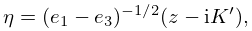
34: 29.2 Differential Equations

… ►This equation has regular singularities at the points $2pK+(2q+1)\mathrm{i}{K}^{\prime }$, where $p,q\in \mathbb{Z}$, and $K$, $K^{\prime }$ are the complete elliptic integrals of the first kind with moduli $k$, $k^{\prime }(={(1-k^2)}^{1/2})$, respectively; see §19.2(ii). … ►

29.2.8 $$\eta ={(e_1-e_3)}^{-1/2}(z-\mathrm{i}{K}^{\prime }),$$

ⓘ

Defines:

$\eta$ (locally)

Symbols:

$K^{\prime }\left(k\right)$: Legendre’s complementary complete elliptic integral of the first kind, $\mathrm{i}$: imaginary unit, $z$: complex variable, $k$: real parameter and $e_j$: constants

Permalink:

http://dlmf.nist.gov/29.2.E8

Encodings:

pMML, png, TeX

See also:

Annotations for §29.2(ii), §29.2 and Ch.29

…

35: 29.18 Mathematical Applications

… ►

$\beta =K+\mathrm{i}{\beta }^{\prime },$

►

$0\le {\beta }^{\prime }\le 2K^{\prime },$

►

$0\le \gamma \le 4K,$

… ►

$\alpha =K+\mathrm{i}{K}^{\prime }-{\alpha }^{\prime },$ ,

►

$\beta =K+\mathrm{i}{\beta }^{\prime },$ $0\le {\beta }^{\prime }\le 2K^{\prime },0\le \gamma \le 4K$,

…

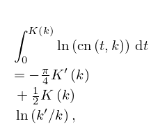
36: 22.14 Integrals

… ►Thirdly, with , … ►Lastly, with , … ►In (22.14.13)–(22.14.15), . … ►

22.14.16 $${\int }_0^{K\left(k\right)}\ln \left(\mathrm{sn}(t,k)\right)dt=-\frac{\pi }{4}{K}^{\prime }\left(k\right)-\frac{1}{2}K\left(k\right)\ln k,$$

ⓘ

Symbols:

$\mathrm{sn}(z,k)$: Jacobian elliptic function, $\pi$: the ratio of the circumference of a circle to its diameter, $K^{\prime }\left(k\right)$: Legendre’s complementary complete elliptic integral of the first kind, $K\left(k\right)$: Legendre’s complete elliptic integral of the first kind, $dx$: differential of $x$ , $\int$: integral, $\ln z$: principal branch of logarithm function and $k$: modulus

Referenced by:

Erratum (V1.0.28) for Equations (22.14.16), (22.14.17)

Permalink:

http://dlmf.nist.gov/22.14.E16

Encodings:

pMML, png, TeX

Correction (effective with 1.0.28):

Originally, a factor of $\pi$ was missing from the term containing the $\frac{1}{4}{K}^{\prime }\left(k\right)$.

Suggested 2020-08-06 by Fred Hucht

See also:

Annotations for §22.14(iv), §22.14 and Ch.22

►

22.14.17 $${\int }_0^{K\left(k\right)}\ln \left(\mathrm{cn}(t,k)\right)dt=-\frac{\pi }{4}{K}^{\prime }\left(k\right)+\frac{1}{2}K\left(k\right)\ln \left(k^{\prime }/k\right),$$

ⓘ

Symbols:

$\mathrm{cn}(z,k)$: Jacobian elliptic function, $\pi$: the ratio of the circumference of a circle to its diameter, $K^{\prime }\left(k\right)$: Legendre’s complementary complete elliptic integral of the first kind, $K\left(k\right)$: Legendre’s complete elliptic integral of the first kind, $dx$: differential of $x$ , $\int$: integral, $\ln z$: principal branch of logarithm function, $k$: modulus and $k^{\prime }$: complementary modulus

Referenced by:

Erratum (V1.0.28) for Equations (22.14.16), (22.14.17)

Permalink:

http://dlmf.nist.gov/22.14.E17

Encodings:

pMML, png, TeX

Correction (effective with 1.0.28):

Originally, a factor of $\pi$ was missing from the term containing the $\frac{1}{4}{K}^{\prime }\left(k\right)$.

Suggested 2020-08-06 by Fred Hucht

See also:

Annotations for §22.14(iv), §22.14 and Ch.22

…

37: 29.12 Definitions

… ►The superscript $m$ on the left-hand sides of (29.12.1)–(29.12.8) agrees with the number of $z$-zeros of each Lamé polynomial in the interval $(0,K)$, while $n-m$ is the number of $z$-zeros in the open line segment from $K$ to $K+\mathrm{i}{K}^{\prime }$. … ►

Table 29.12.1: Lamé polynomials.

► ►►►►►

$\nu$	eigenvalue $h$	eigenfunction $w(z)$	polynomial form	real period	imag. period	parity of $w(z)$	parity of $w(z-K)$	parity of $w(z-K-\mathrm{i}{K}^{\prime })$
$2n$	$a_{\nu }^{2m}\left(k^2\right)$	${\mathrm{𝑢𝐸}}_{\nu }^m(z,k^2)$	$P({\mathrm{sn}}^2)$	$2K$	$2\mathrm{i}{K}^{\prime }$	even	even	even
…
$2n+2$	$b_{\nu }^{2m+2}\left(k^2\right)$	${\mathrm{𝑠𝑐𝐸}}_{\nu }^m(z,k^2)$	$\mathrm{sn}\mathrm{cn}P({\mathrm{sn}}^2)$	$2K$	$4\mathrm{i}{K}^{\prime }$	odd	odd	even
…
$2n+3$	$b_{\nu }^{2m+2}\left(k^2\right)$	${\mathrm{𝑠𝑐𝑑𝐸}}_{\nu }^m(z,k^2)$	$\mathrm{sn}\mathrm{cn}\mathrm{dn}P({\mathrm{sn}}^2)$	$2K$	$2\mathrm{i}{K}^{\prime }$	odd	odd	odd

►

…

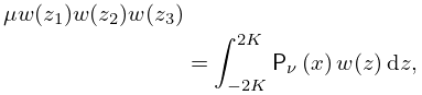
38: 29.8 Integral Equations

… ►Let $w(z)$ be any solution of (29.2.1) of period $4K$, $w_2(z)$ be a linearly independent solution, and $𝒲\left\{w,w_2\right\}$ denote their Wronskian. … ►

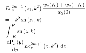
29.8.2 $$\mu w(z_1)w(z_2)w(z_3)={\int }_{-2K}^{2K}{𝖯}_{\nu }\left(x\right)w(z)dz,$$

ⓘ

Symbols:

$K\left(k\right)$: Legendre’s complete elliptic integral of the first kind, $dx$: differential of $x$ , $\int$: integral, ${𝖯}_{\nu }\left(x\right)={𝖯}_{\nu }^0\left(x\right)$: Ferrers function of the first kind, $x$: real variable, $z$: complex variable, $k$: real parameter, $\nu$: real parameter, $w(z)$: solution and $\mu$

Referenced by:

§29.8

Permalink:

http://dlmf.nist.gov/29.8.E2

Encodings:

pMML, png, TeX

See also:

Annotations for §29.8 and Ch.29

… ►

$$w(z+2K)=\sigma w(z),$$

►

$$w_2(z+2K)=\tau w(z)+\sigma w_2(z).$$

… ►

29.8.7 $${\mathrm{𝐸𝑐}}_{\nu }^{2m+1}(z_1,k^2)\frac{w_2(K)+w_2(-K)}{w_2(0)}=-k^2\mathrm{sn}(z_1,k){\int }_{-K}^K\mathrm{sn}(z,k)\frac{d{𝖯}_{\nu }\left(y\right)}{dy}{\mathrm{𝐸𝑐}}_{\nu }^{2m+1}(z,k^2)dz,$$

ⓘ

Symbols:

$\mathrm{sn}(z,k)$: Jacobian elliptic function, ${\mathrm{𝐸𝑐}}_{\nu }^m(z,k^2)$: Lamé function, $K\left(k\right)$: Legendre’s complete elliptic integral of the first kind, $\frac{df}{dx}$: derivative of $f$ with respect to $x$ , $dx$: differential of $x$ , $\int$: integral, ${𝖯}_{\nu }\left(x\right)={𝖯}_{\nu }^0\left(x\right)$: Ferrers function of the first kind, $m$: nonnegative integer, $y$: real variable, $z$: complex variable, $k$: real parameter, $\nu$: real parameter and $w(z)$: solution

Permalink:

http://dlmf.nist.gov/29.8.E7

Encodings:

pMML, png, TeX

See also:

Annotations for §29.8 and Ch.29

…

39: 36.1 Special Notation

… ►The main functions covered in this chapter are cuspoid catastrophes ${\mathrm{\Phi }}_K(t;𝐱)$; umbilic catastrophes with codimension three ${\mathrm{\Phi }}^{(\mathrm{E})}(s,t;𝐱)$, ${\mathrm{\Phi }}^{(\mathrm{H})}(s,t;𝐱)$; canonical integrals ${\mathrm{\Psi }}_K\left(𝐱\right)$, ${\mathrm{\Psi }}^{(\mathrm{E})}\left(𝐱\right)$, ${\mathrm{\Psi }}^{(\mathrm{H})}\left(𝐱\right)$; diffraction catastrophes ${\mathrm{\Psi }}_K(𝐱;k)$, ${\mathrm{\Psi }}^{(\mathrm{E})}(𝐱;k)$, ${\mathrm{\Psi }}^{(\mathrm{H})}(𝐱;k)$ generated by the catastrophes. …

40: 22.18 Mathematical Applications

… ►where $k=\sqrt{1-(b^2/a^2)}$ is the eccentricity, and $0\le u\le 4K\left(k\right)$. … ►With $k\in [0,1]$ the mapping $z\to w=\mathrm{sn}(z,k)$ gives a conformal map of the closed rectangle $[-K,K]\times [0,K^{\prime }]$ onto the half-plane $\mathrm{\Im }w\ge 0$, with $0,\pm K,\pm K+\mathrm{i}{K}^{\prime },\mathrm{i}{K}^{\prime }$ mapping to $0,\pm 1,\pm k^{-2},\mathrm{\infty }$ respectively. The half-open rectangle $(-K,K)\times [-K^{\prime },K^{\prime }]$ maps onto $ℂ$ cut along the intervals $(-\mathrm{\infty },-1]$ and $[1,\mathrm{\infty })$. …