elliptic form

SearchAdvancedHelp

(0.003 seconds)

11—20 of 51 matching pages

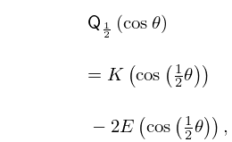
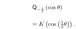
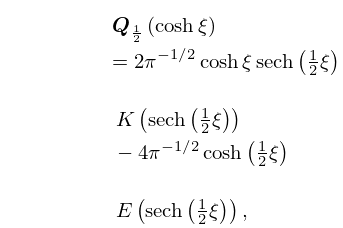
11: 14.5 Special Values

… ►

14.5.20 $${𝖯}_{\frac{1}{2}}\left(\cos \theta \right)=\frac{2}{\pi }\left(2E\left(\sin \left(\frac{1}{2}\theta \right)\right)-K\left(\sin \left(\frac{1}{2}\theta \right)\right)\right),$$

ⓘ

Symbols:

$\pi$: the ratio of the circumference of a circle to its diameter, $K\left(k\right)$: Legendre’s complete elliptic integral of the first kind, $E\left(k\right)$: Legendre’s complete elliptic integral of the second kind, $\cos z$: cosine function, ${𝖯}_{\nu }\left(x\right)={𝖯}_{\nu }^0\left(x\right)$: Ferrers function of the first kind, $\sin z$: sine function and : variable

A&S Ref:

8.13.11 (in slightly different form)

Permalink:

http://dlmf.nist.gov/14.5.E20

Encodings:

pMML, png, TeX

See also:

Annotations for §14.5(v), §14.5 and Ch.14

… ►

14.5.22 $${𝖰}_{\frac{1}{2}}\left(\cos \theta \right)=K\left(\cos \left(\frac{1}{2}\theta \right)\right)-2E\left(\cos \left(\frac{1}{2}\theta \right)\right),$$

ⓘ

Symbols:

$K\left(k\right)$: Legendre’s complete elliptic integral of the first kind, $E\left(k\right)$: Legendre’s complete elliptic integral of the second kind, $\cos z$: cosine function, ${𝖰}_{\nu }\left(x\right)={𝖰}_{\nu }^0\left(x\right)$: Ferrers function of the second kind and : variable

A&S Ref:

8.13.12 (in slightly different form)

Permalink:

http://dlmf.nist.gov/14.5.E22

Encodings:

pMML, png, TeX

See also:

Annotations for §14.5(v), §14.5 and Ch.14

►

14.5.23 $${𝖰}_{-\frac{1}{2}}\left(\cos \theta \right)=K\left(\cos \left(\frac{1}{2}\theta \right)\right).$$

ⓘ

Symbols:

$K\left(k\right)$: Legendre’s complete elliptic integral of the first kind, $\cos z$: cosine function, ${𝖰}_{\nu }\left(x\right)={𝖰}_{\nu }^0\left(x\right)$: Ferrers function of the second kind and : variable

A&S Ref:

8.13.10 (in slightly different form)

Permalink:

http://dlmf.nist.gov/14.5.E23

Encodings:

pMML, png, TeX

See also:

Annotations for §14.5(v), §14.5 and Ch.14

… ►

14.5.26 $${𝑸}_{\frac{1}{2}}\left(\cosh \xi \right)=2{\pi }^{-1/2}\cosh \xi \mathrm{sech}\left(\frac{1}{2}\xi \right)K\left(\mathrm{sech}\left(\frac{1}{2}\xi \right)\right)-4{\pi }^{-1/2}\cosh \left(\frac{1}{2}\xi \right)E\left(\mathrm{sech}\left(\frac{1}{2}\xi \right)\right),$$

ⓘ

Symbols:

$\pi$: the ratio of the circumference of a circle to its diameter, $K\left(k\right)$: Legendre’s complete elliptic integral of the first kind, $E\left(k\right)$: Legendre’s complete elliptic integral of the second kind, $\cosh z$: hyperbolic cosine function, $\mathrm{sech}z$: hyperbolic secant function, ${𝑸}_{\nu }\left(z\right)={𝑸}_{\nu }^0\left(z\right)$: Olver’s associated Legendre function and $\xi >0$: variable

A&S Ref:

8.13.7 (in slightly different form)

Permalink:

http://dlmf.nist.gov/14.5.E26

Encodings:

pMML, png, TeX

See also:

Annotations for §14.5(v), §14.5 and Ch.14

…

12: Bille C. Carlson

… ►In Symmetry in c, d, n of Jacobian elliptic functions (2004) he found a previously hidden symmetry in relations between Jacobian elliptic functions, which can now take a form that remains valid when the letters c, d, and n are permuted. …

13: Bibliography K

… ►

Introduction to Elliptic Curves and Modular Forms. 2nd edition, Graduate Texts in Mathematics, Vol. 97, Springer-Verlag, New York.

ⓘ

External Links:

ISBN 0-387-97966-2, MathReview, ZentralBlatt

Referenced by:

§20.10(i), §20.12(i), §20.9(iii), §22.18(iv), §23.1, §23.20(ii), §23.20(v), Ch.23.

Encodings:

BibTeX

…

14: 19.16 Definitions

… ►All elliptic integrals of the form (19.2.3) and many multiple integrals, including (19.23.6) and (19.23.6_5), are special cases of a multivariate hypergeometric function …

15: Bibliography L

… ►

Reduction of Elliptic Integrals to Legendre Normal Form. Technical report Technical Report 97-21, Department of Computer Science, University of Waterloo, Waterloo, Ontario.

ⓘ

Referenced by:

§19.14(ii).

Encodings:

BibTeX

…

16: Errata

… ►

Originally the limiting form for $\mathrm{sc}(z,k)$ in the last line of this table was incorrect ($\cosh z$, instead of $\sinh z$).

$\mathrm{sn}(z,k)$ $\to$	$\tanh z$	$\mathrm{cd}(z,k)$ $\to$	$1$	$\mathrm{dc}(z,k)$ $\to$	$1$	$\mathrm{ns}(z,k)$ $\to$	$\coth z$
$\mathrm{cn}(z,k)$ $\to$	$\mathrm{sech}z$	$\mathrm{sd}(z,k)$ $\to$	$\sinh z$	$\mathrm{nc}(z,k)$ $\to$	$\cosh z$	$\mathrm{ds}(z,k)$ $\to$	$\mathrm{csch}z$
$\mathrm{dn}(z,k)$ $\to$	$\mathrm{sech}z$	$\mathrm{nd}(z,k)$ $\to$	$\cosh z$	$\mathrm{sc}(z,k)$ $\to$	$\sinh z$	$\mathrm{cs}(z,k)$ $\to$	$\mathrm{csch}z$

Reported 2010-11-23.

…

17: Mathematical Introduction

… ►Other examples are: (a) the notation for the Ferrers functions—also known as associated Legendre functions on the cut—for which existing notations can easily be confused with those for other associated Legendre functions (§14.1); (b) the spherical Bessel functions for which existing notations are unsymmetric and inelegant (§§10.47(i) and 10.47(ii)); and (c) elliptic integrals for which both Legendre’s forms and the more recent symmetric forms are treated fully (Chapter 19). …

18: 28.33 Physical Applications

… ►

Boundary-values problems arising from solution of the two-dimensional wave equation in elliptical coordinates. This yields a pair of equations of the form (28.2.1) and (28.20.1), and the appropriate solution of (28.2.1) is usually a periodic solution of integer order. See §28.33(ii).

…

19: 29.15 Fourier Series and Chebyshev Series

… ►Since (29.2.5) implies that $\cos \varphi =\mathrm{sn}(z,k)$, (29.15.1) can be rewritten in the form …

20: 29.14 Orthogonality

… ►

29.14.2 $$⟨g,h⟩={\int }_0^K{\int }_0^{K^{\prime }}w(s,t)g(s,t)h(s,t)dtds,$$

ⓘ

Symbols:

$K^{\prime }\left(k\right)$: Legendre’s complementary complete elliptic integral of the first kind, $K\left(k\right)$: Legendre’s complete elliptic integral of the first kind, $dx$: differential of $x$ , $\int$: integral, $k$: real parameter and $w(s,t)$: function

Referenced by:

§29.14

Permalink:

http://dlmf.nist.gov/29.14.E2

Encodings:

pMML, png, TeX

See also:

Annotations for §29.14 and Ch.29

… ►

29.14.3 $$w(s,t)={\mathrm{sn}}^2(K+\mathrm{i}t,k)-{\mathrm{sn}}^2(s,k).$$

ⓘ

Symbols:

$\mathrm{sn}(z,k)$: Jacobian elliptic function, $K\left(k\right)$: Legendre’s complete elliptic integral of the first kind, $\mathrm{i}$: imaginary unit, $k$: real parameter and $w(s,t)$: function

Referenced by:

§29.14

Permalink:

http://dlmf.nist.gov/29.14.E3

Encodings:

pMML, png, TeX

See also:

Annotations for §29.14 and Ch.29

… ►

29.14.4 $${\mathrm{𝑠𝐸}}_{2n+1}^m(s,k^2){\mathrm{𝑠𝐸}}_{2n+1}^m(K+\mathrm{i}t,k^2),$$

ⓘ

Symbols:

${\mathrm{𝑠𝐸}}_{2n+1}^m(z,k^2)$: Lamé polynomial, $K\left(k\right)$: Legendre’s complete elliptic integral of the first kind, $\mathrm{i}$: imaginary unit, $m$: nonnegative integer, $n$: nonnegative integer and $k$: real parameter

Referenced by:

§29.14

Permalink:

http://dlmf.nist.gov/29.14.E4

Encodings:

pMML, png, TeX

See also:

Annotations for §29.14 and Ch.29

… ►When combined, all eight systems (29.14.1) and (29.14.4)–(29.14.10) form an orthogonal and complete system with respect to the inner product ►

29.14.11 $$⟨g,h⟩={\int }_0^{4K}{\int }_0^{2K^{\prime }}w(s,t)g(s,t)h(s,t)dtds,$$

ⓘ

Symbols:

$K^{\prime }\left(k\right)$: Legendre’s complementary complete elliptic integral of the first kind, $K\left(k\right)$: Legendre’s complete elliptic integral of the first kind, $dx$: differential of $x$ , $\int$: integral, $k$: real parameter and $w(s,t)$: function

Permalink:

http://dlmf.nist.gov/29.14.E11

Encodings:

pMML, png, TeX

See also:

Annotations for §29.14 and Ch.29

…