cut

SearchAdvancedHelp

(0.001 seconds)

11—20 of 66 matching pages

11: 30.18 Software

… ►

SWF2: ${\mathrm{𝖯𝗌}}_n^m(x,{\gamma }^2)$.

►

SWF3: ${\mathrm{𝖰𝗌}}_n^m(x,{\gamma }^2)$.

…

12: 10.72 Mathematical Applications

… ►These expansions are uniform with respect to $z$, including the turning point $z_0$ and its neighborhood, and the region of validity often includes cut neighborhoods (§1.10(vi)) of other singularities of the differential equation, especially irregular singularities. … ►These asymptotic expansions are uniform with respect to $z$, including cut neighborhoods of $z_0$, and again the region of uniformity often includes cut neighborhoods of other singularities of the differential equation. … ►These approximations are uniform with respect to both $z$ and $\alpha$, including $z=z_0(a)$, the cut neighborhood of $z=0$, and $\alpha =a$. …

13: 14.27 Zeros

… ► $P_{\nu }^{\mu }\left(x\pm \mathrm{i}0\right)$ (either side of the cut) has exactly one zero in the interval $(-\mathrm{\infty },-1)$ if either of the following sets of conditions holds: …

14: 4.25 Continued Fractions

… ►valid when $z$ lies in the open cut plane shown in Figure 4.23.1(i). …valid when $z$ lies in the open cut plane shown in Figure 4.23.1(ii). …valid when $z$ lies in the open cut plane shown in Figure 4.23.1(iv). …

15: 4.3 Graphics

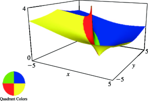
… ►Figure 4.3.2 illustrates the conformal mapping of the strip onto the whole $w$-plane cut along the negative real axis, where $w={\mathrm{e}}^z$ and $z=\ln w$ (principal value). … ►

►

►

Figure 4.3.3: $\ln \left(x+\mathrm{i}y\right)$ (principal value). There is a branch cut along the negative real axis. Magnify 3D Help

…

16: Philip J. Davis

… ►Moreover, a cutting plane feature allows users to track curves of intersection produced as a moving plane cuts through the function surface. …

17: 30.16 Methods of Computation

… ►If $|{\gamma }^2|$ is large, then we can use the asymptotic expansions referred to in §30.9 to approximate ${\mathrm{𝖯𝗌}}_n^m(x,{\gamma }^2)$. ►If ${\lambda }_n^m\left({\gamma }^2\right)$ is known, then we can compute ${\mathrm{𝖯𝗌}}_n^m(x,{\gamma }^2)$ (not normalized) by solving the differential equation (30.2.1) numerically with initial conditions $w(0)=1$, $w^{\prime }(0)=0$ if $n-m$ is even, or $w(0)=0$, $w^{\prime }(0)=1$ if $n-m$ is odd. ►If ${\lambda }_n^m\left({\gamma }^2\right)$ is known, then ${\mathrm{𝖯𝗌}}_n^m(x,{\gamma }^2)$ can be found by summing (30.8.1). … ►

30.16.9 $${\mathrm{𝖯𝗌}}_n^m(x,{\gamma }^2)=\underset{d\to \mathrm{\infty }}{lim}\sum _{j=1}^d{(-1)}^{j-p}{e}_{j,d}{𝖯}_{n+2(j-p)}^m\left(x\right).$$

ⓘ

Symbols:

: Ferrers function of the first kind, ${\mathrm{𝖯𝗌}}_n^m(x,{\gamma }^2)$: spheroidal wave function of the first kind, $x$: real variable, $m$: nonnegative integer, $n\ge m$: integer degree, $d$: dimension and ${\gamma }^2$: real parameter

Permalink:

http://dlmf.nist.gov/30.16.E9

Encodings:

pMML, png, TeX

See also:

Annotations for §30.16(ii), §30.16 and Ch.30

…

18: 4.23 Inverse Trigonometric Functions

… ►These functions are analytic in the cut plane depicted in Figures 4.23.1(iii) and 4.23.1(iv). … ►

§4.23(iv) Logarithmic Forms

… ►On the cuts … ►On the cuts … ►On the cuts …

19: 30.8 Expansions in Series of Ferrers Functions

… ►

30.8.1 $${\mathrm{𝖯𝗌}}_n^m(x,{\gamma }^2)=\sum _{k=-R}^{\mathrm{\infty }}{(-1)}^k{a}_{n,k}^m({\gamma }^2){𝖯}_{n+2k}^m\left(x\right),$$

ⓘ

Symbols:

: Ferrers function of the first kind, ${\mathrm{𝖯𝗌}}_n^m(x,{\gamma }^2)$: spheroidal wave function of the first kind, $x$: real variable, $m$: nonnegative integer, $n\ge m$: integer degree, ${\gamma }^2$: real parameter, $R=\lfloor (n-m)/2\rfloor$: limit and $a_{n,k}^m({\gamma }^2)$: coefficients

A&S Ref:

21.7.1 (in different form)

Referenced by:

§30.16(ii), §30.16(ii)

Permalink:

http://dlmf.nist.gov/30.8.E1

Encodings:

pMML, png, TeX

See also:

Annotations for §30.8(i), §30.8 and Ch.30

… ►

30.8.2 $$a_{n,k}^m({\gamma }^2)={(-1)}^k\left(n+2k+\frac{1}{2}\right)\frac{(n-m+2k)!}{(n+m+2k)!}{\int }_{-1}^1{\mathrm{𝖯𝗌}}_n^m(x,{\gamma }^2){𝖯}_{n+2k}^m\left(x\right)dx.$$

ⓘ

Defines:

$a_{n,k}^m({\gamma }^2)$: coefficients (locally)

Symbols:

: Ferrers function of the first kind, $dx$: differential of $x$ , $!$: factorial (as in $n!$), $\int$: integral, ${\mathrm{𝖯𝗌}}_n^m(x,{\gamma }^2)$: spheroidal wave function of the first kind, $x$: real variable, $m$: nonnegative integer, $n\ge m$: integer degree and ${\gamma }^2$: real parameter

Referenced by:

§30.11(i)

Permalink:

http://dlmf.nist.gov/30.8.E2

Encodings:

pMML, png, TeX

See also:

Annotations for §30.8(i), §30.8 and Ch.30

… ►

30.8.9 $${\mathrm{𝖰𝗌}}_n^m(x,{\gamma }^2)=\sum _{k=-\mathrm{\infty }}^{-N-1}{(-1)}^{k}a_{}^{\prime }{}_{n,k}{}^m({\gamma }^2){𝖯}_{n+2k}^m\left(x\right)+\sum _{k=-N}^{\mathrm{\infty }}{(-1)}^k{a}_{n,k}^m({\gamma }^2){𝖰}_{n+2k}^m\left(x\right),$$

ⓘ

Symbols:

: Ferrers function of the first kind, : Ferrers function of the second kind, ${\mathrm{𝖰𝗌}}_n^m(x,{\gamma }^2)$: spheroidal wave function of the second kind, $x$: real variable, $m$: nonnegative integer, $n\ge m$: integer degree, ${\gamma }^2$: real parameter, $a_{n,k}^m({\gamma }^2)$: coefficients and $N$: upper limit

A&S Ref:

21.7.21 (in different form)

Permalink:

http://dlmf.nist.gov/30.8.E9

Encodings:

pMML, png, TeX

See also:

Annotations for §30.8(ii), §30.8 and Ch.30

… ►It should be noted that if the forward recursion (30.8.4) beginning with $f_{-N-1}=0$, $f_{-N}=1$ leads to $f_{-R}=0$, then $a_{n,k}^m({\gamma }^2)$ is undefined for and ${\mathrm{𝖰𝗌}}_n^m(x,{\gamma }^2)$ does not exist. …

20: 14.1 Special Notation

… ►The main functions treated in this chapter are the Legendre functions ${𝖯}_{\nu }\left(x\right)$, ${𝖰}_{\nu }\left(x\right)$, $P_{\nu }\left(z\right)$, $Q_{\nu }\left(z\right)$; Ferrers functions ${𝖯}_{\nu }^{\mu }\left(x\right)$, ${𝖰}_{\nu }^{\mu }\left(x\right)$ (also known as the Legendre functions on the cut); associated Legendre functions $P_{\nu }^{\mu }\left(z\right)$, $Q_{\nu }^{\mu }\left(z\right)$, ${𝑸}_{\nu }^{\mu }\left(z\right)$; conical functions ${𝖯}_{-\frac{1}{2}+\mathrm{i}\tau }^{\mu }\left(x\right)$, ${𝖰}_{-\frac{1}{2}+\mathrm{i}\tau }^{\mu }\left(x\right)$, ${\widehat{𝖰}}_{-\frac{1}{2}+\mathrm{i}\tau }^{\mu }\left(x\right)$, $P_{-\frac{1}{2}+\mathrm{i}\tau }^{\mu }\left(x\right)$, $Q_{-\frac{1}{2}+\mathrm{i}\tau }^{\mu }\left(x\right)$ (also known as Mehler functions). …