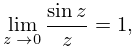
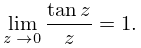
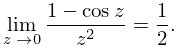
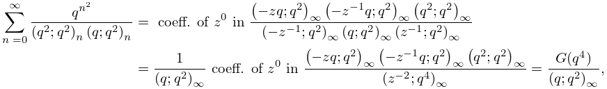
as z→0
(0.031 seconds)
21—30 of 616 matching pages
21: 19.21 Connection Formulas
…
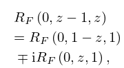
►Upper signs apply if , and lower signs if :
►
19.21.4
…
►If and , then as (19.21.6) reduces to Legendre’s relation (19.21.1).
…
►Because is completely symmetric, can be permuted on the right-hand side of (19.21.10) so that if the variables are real, thereby avoiding cancellations when is calculated from and (see §19.36(i)).
…
►Let be real and nonnegative, with at most one of them 0.
…
22: 1.9 Calculus of a Complex Variable
…
►and when ,
…
►A function is continuous at a point if .
…
►( may or may not belong to .)
…
►A function is said to be analytic (holomorphic) at if it is complex differentiable in a neighborhood of .
…
►where is an integer called the winding number of
with respect to
.
…
23: 10.2 Definitions
…
►This solution of (10.2.1) is an analytic function of , except for a branch point at when is not an integer.
…
►For fixed
each branch of is entire in .
…
►Whether or not is an integer has a branch point at .
…
►For fixed
each branch of is entire in .
…
►Each solution has a branch point at for all .
…
24: 14.28 Sums
…
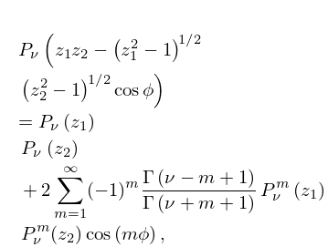
►When , , , and ,
►
14.28.1
►where the branches of the square roots have their principal values when and are continuous when .
…
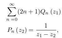
►
14.28.2
, ,
…
25: 10.30 Limiting Forms
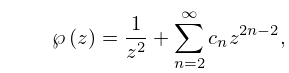
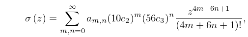
26: 23.9 Laurent and Other Power Series
…
►Let be the nearest lattice point to the origin, and define
…
►
23.9.2
,
►
23.9.3
.
…
►Also, Abramowitz and Stegun (1964, (18.5.25)) supplies the first 22 terms in the reverted form of (23.9.2) as .
…
►
23.9.7
…
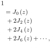
27: 10.12 Generating Function and Associated Series
28: 3.8 Nonlinear Equations
…
►If and , then is a simple zero of .
If and , then is a zero of of multiplicity
; compare §1.10(i).
…
►An iterative method converges locally to a solution if there exists a neighborhood of such that whenever the initial approximation lies within .
…
►The results for are given in Table 3.8.2.
…
►For an arbitrary starting point , convergence cannot be predicted, and the boundary of the set of points that generate a sequence converging to a particular zero has a very complicated structure.
…
