as%20z%E2%86%920

SearchAdvancedHelp

(0.004 seconds)

1—10 of 768 matching pages

1: 20 Theta Functions

Chapter 20 Theta Functions

…

2: 6.19 Tables

… ►

Zhang and Jin (1996, pp. 652, 689) includes $\mathrm{Si}\left(x\right)$, $\mathrm{Ci}\left(x\right)$, $x=0(.5)20(2)30$, 8D; $\mathrm{Ei}\left(x\right)$, $E_1\left(x\right)$, $x=[0,100]$, 8S.

►

§6.19(iii) Complex Variables, $z=x+\mathrm{i}y$

►

Abramowitz and Stegun (1964, Chapter 5) includes the real and imaginary parts of $z{\mathrm{e}}^z{E}_1\left(z\right)$, $x=-19(1)20$, $y=0(1)20$, 6D; ${\mathrm{e}}^z{E}_1\left(z\right)$, $x=-4(.5)-2$, $y=0(.2)1$, 6D; $E_1\left(z\right)+\ln z$, $x=-2(.5)2.5$, $y=0(.2)1$, 6D.

►

Zhang and Jin (1996, pp. 690–692) includes the real and imaginary parts of $E_1\left(z\right)$, $\pm x=0.5,1,3,5,10,15,20,50,100$, $y=0(.5)1(1)5(5)30,50,100$, 8S.

3: 10.75 Tables

… ►

Zhang and Jin (1996, pp. 185–195) tabulates $J_n\left(x\right)$, $J_n^{\prime }\left(x\right)$, $Y_n\left(x\right)$, $Y_n^{\prime }\left(x\right)$, $n=0(1)10(10)50,100$, $x=1$, 5, 10, 25, 50, 100, 9S; $J_{n+\alpha }\left(x\right)$, $J_{n+\alpha }^{\prime }\left(x\right)$, $Y_{n+\alpha }\left(x\right)$, $Y_{n+\alpha }^{\prime }\left(x\right)$, $n=0(1)5,10,30,50,100$, $\alpha =\frac{1}{4},\frac{1}{3},\frac{1}{2},\frac{2}{3},\frac{3}{4}$, $x=1,5,10,50$, 8S; real and imaginary parts of $J_{n+\alpha }\left(z\right)$, $J_{n+\alpha }^{\prime }\left(z\right)$, $Y_{n+\alpha }\left(z\right)$, $Y_{n+\alpha }^{\prime }\left(z\right)$, $n=0(1)15,20(10)50,100$, $\alpha =0,\frac{1}{2}$, $z=4+2\mathrm{i}$, $20+10\mathrm{i}$, 8S.

… ►

Bickley et al. (1952) tabulates $x^{-n}{I}_n\left(x\right)$ or ${\mathrm{e}}^{-x}{I}_n\left(x\right)$, $x^n{K}_n\left(x\right)$ or ${\mathrm{e}}^x{K}_n\left(x\right)$, $n=2(1)20$, $x=0$(.01 or .1) 10(.1) 20, 8S; $I_n\left(x\right)$, $K_n\left(x\right)$, $n=0(1)20$, $x=0$ or $0.1(.1)20$, 10S.

… ►

Zhang and Jin (1996, pp. 240–250) tabulates $I_n\left(x\right)$, $I_n^{\prime }\left(x\right)$, $K_n\left(x\right)$, $K_n^{\prime }\left(x\right)$, $n=0(1)10(10)50,100$, $x=1,5,10,25,50,100$, 9S; $I_{n+\alpha }\left(x\right)$, $I_{n+\alpha }^{\prime }\left(x\right)$, $K_{n+\alpha }\left(x\right)$, $K_{n+\alpha }^{\prime }\left(x\right)$, $n=0(1)5$, 10, 30, 50, 100, $\alpha =\frac{1}{4}$, $\frac{1}{3}$, $\frac{1}{2}$, $\frac{2}{3}$, $\frac{3}{4}$, $x=1$, 5, 10, 50, 8S; real and imaginary parts of $I_{n+\alpha }\left(z\right)$, $I_{n+\alpha }^{\prime }\left(z\right)$, $K_{n+\alpha }\left(z\right)$, $K_{n+\alpha }^{\prime }\left(z\right)$, $n=0(1)15$, 20(10)50, 100, $\alpha =0,\frac{1}{2}$, $z=4+2\mathrm{i},20+10\mathrm{i}$, 8S.

… ►

Kerimov and Skorokhodov (1984b) tabulates all zeros of the principal values of $K_n\left(z\right)$ and $K_n^{\prime }\left(z\right)$, for $n=2(1)20$, 9S.

►

Kerimov and Skorokhodov (1984c) tabulates all zeros of $I_{-n-\frac{1}{2}}\left(z\right)$ and $I_{-n-\frac{1}{2}}^{\prime }\left(z\right)$ in the sector $0\le \mathrm{ph}z\le \frac{1}{2}\pi$ for $n=1(1)20$, 9S.

…

4: 6.20 Approximations

… ►

Cody and Thacher (1968) provides minimax rational approximations for $E_1\left(x\right)$, with accuracies up to 20S.

►

Cody and Thacher (1969) provides minimax rational approximations for $\mathrm{Ei}\left(x\right)$, with accuracies up to 20S.

►

MacLeod (1996b) provides rational approximations for the sine and cosine integrals and for the auxiliary functions $\mathrm{f}$ and $\mathrm{g}$, with accuracies up to 20S.

… ►

Luke (1969b, pp. 402, 410, and 415–421) gives main diagonal Padé approximations for $\mathrm{Ein}\left(z\right)$, $\mathrm{Si}\left(z\right)$, $\mathrm{Cin}\left(z\right)$ (valid near the origin), and $E_1\left(z\right)$ (valid for large $|z|$); approximate errors are given for a selection of $z$-values.

►

Luke (1969b, pp. 411–414) gives rational approximations for $\mathrm{Ein}\left(z\right)$.

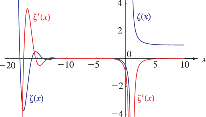
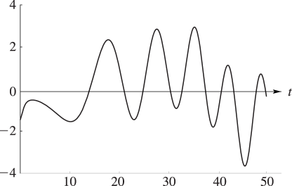
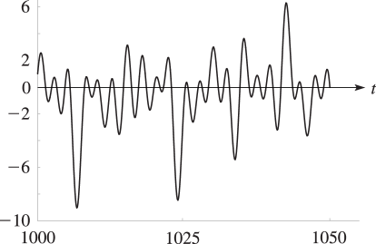
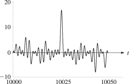
5: 25.12 Polylogarithms

… ►Other notations and names for ${\mathrm{Li}}_2\left(z\right)$ include $S_2(z)$ (Kölbig et al. (1970)), Spence function $\mathrm{Sp}(z)$ (’t Hooft and Veltman (1979)), and ${\mathrm{L}}_2(z)$ (Maximon (2003)). ►In the complex plane ${\mathrm{Li}}_2\left(z\right)$ has a branch point at $z=1$. … ►For real or complex $s$ and $z$ the polylogarithm ${\mathrm{Li}}_s\left(z\right)$ is defined by … ►For each fixed complex $s$ the series defines an analytic function of $z$ for . …For other values of $z$, ${\mathrm{Li}}_s\left(z\right)$ is defined by analytic continuation. …

6: 25.3 Graphics

… ►

►►

Figure 25.3.1: Riemann zeta function $\zeta \left(x\right)$ and its derivative ${\zeta }^{\prime }\left(x\right)$, $-20\le x\le 10$. Magnify

… ►

►►

Figure 25.3.4: $Z(t)$, $0\le t\le 50$. $Z(t)$ and $\zeta \left(\frac{1}{2}+\mathrm{i}t\right)$ have the same zeros. … Magnify

►

►►

Figure 25.3.5: $Z(t)$, $1000\le t\le 1050$. Magnify

►

►►

Figure 25.3.6: $Z(t)$, $10000\le t\le 10050$. Magnify

7: 7.24 Approximations

… ►

Cody (1969) provides minimax rational approximations for $\mathrm{erf}x$ and $\mathrm{erfc}x$. The maximum relative precision is about 20S.

… ►

Cody et al. (1970) gives minimax rational approximations to Dawson’s integral $F\left(x\right)$ (maximum relative precision 20S–22S).

… ►

Luke (1969b, vol. 2, pp. 422–435) gives main diagonal Padé approximations for $F\left(z\right)$, $\mathrm{erf}z$, $\mathrm{erfc}z$, $C\left(z\right)$, and $S\left(z\right)$; approximate errors are given for a selection of $z$-values.

8: 8 Incomplete Gamma and Related
Functions

…

9: 28 Mathieu Functions and Hill’s Equation

…

10: 9.18 Tables

… ►

Miller (1946) tabulates $\mathrm{Ai}\left(x\right)$, ${\mathrm{Ai}}^{\prime }\left(x\right)$ for $x=-20(.01)2;$ ${\log }_{10}\mathrm{Ai}\left(x\right)$, ${\mathrm{Ai}}^{\prime }\left(x\right)/\mathrm{Ai}\left(x\right)$ for $x=0(.1)25(1)75$; $\mathrm{Bi}\left(x\right)$, ${\mathrm{Bi}}^{\prime }\left(x\right)$ for $x=-10(.1)2.5$; ${\log }_{10}\mathrm{Bi}\left(x\right)$, ${\mathrm{Bi}}^{\prime }\left(x\right)/\mathrm{Bi}\left(x\right)$ for $x=0(.1)10$; $M\left(x\right)$, $N\left(x\right)$, $\theta \left(x\right)$, $\varphi \left(x\right)$ (respectively $F(x)$, $G(x)$, $\chi (x)$, $\psi (x)$) for $x=-80(1)-30(.1)0$. Precision is generally 8D; slightly less for some of the auxiliary functions. Extracts from these tables are included in Abramowitz and Stegun (1964, Chapter 10), together with some auxiliary functions for large arguments.

… ►

Zhang and Jin (1996, p. 337) tabulates $\mathrm{Ai}\left(x\right)$, ${\mathrm{Ai}}^{\prime }\left(x\right)$, $\mathrm{Bi}\left(x\right)$, ${\mathrm{Bi}}^{\prime }\left(x\right)$ for $x=0(1)20$ to 8S and for $x=-20(1)0$ to 9D.

… ►

Miller (1946) tabulates $a_k$, ${\mathrm{Ai}}^{\prime }\left(a_k\right)$, $a_k^{\prime }$, $\mathrm{Ai}\left(a_k^{\prime }\right)$, $k=1(1)50$; $b_k$, ${\mathrm{Bi}}^{\prime }\left(b_k\right)$, $b_k^{\prime }$, $\mathrm{Bi}\left(b_k^{\prime }\right)$, $k=1(1)20$. Precision is 8D. Entries for $k=1(1)20$ are reproduced in Abramowitz and Stegun (1964, Chapter 10).

►

Sherry (1959) tabulates $a_k$, ${\mathrm{Ai}}^{\prime }\left(a_k\right)$, $a_k^{\prime }$, $\mathrm{Ai}\left(a_k^{\prime }\right)$, $k=1(1)50$; 20S.

►

Zhang and Jin (1996, p. 339) tabulates $a_k$, ${\mathrm{Ai}}^{\prime }\left(a_k\right)$, $a_k^{\prime }$, $\mathrm{Ai}\left(a_k^{\prime }\right)$, $b_k$, ${\mathrm{Bi}}^{\prime }\left(b_k\right)$, $b_k^{\prime }$, $\mathrm{Bi}\left(b_k^{\prime }\right)$, $k=1(1)20$; 8D.

…