arithmetic-geometric mean

(0.002 seconds)

9 matching pages

1: 19.8 Quadratic Transformations

… ►

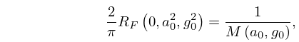
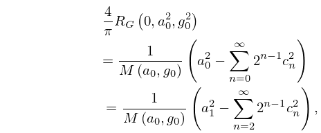
§19.8(i) Gauss’s Arithmetic-Geometric Mean (AGM)

… ►As

n\to\infty

a_{n}

and

g_{n}

converge to a common limit

M\left(a_{0},g_{0}\right)

called the AGM (Arithmetic-Geometric Mean) of

a_{0}

and

g_{0}

. …showing that the convergence of

c_{n}

to 0 and of

a_{n}

and

g_{n}

M\left(a_{0},g_{0}\right)

is quadratic in each case. … ►

19.8.5

K\left(k\right)=\frac{\pi}{2M\left(1,k^{\prime}\right)},

-\infty<k^{2}<1

ⓘ

Symbols:: $M\left(\NVar{a},\NVar{g}\right)$ : arithmetic-geometric mean, $\pi$ : the ratio of the circumference of a circle to its diameter, $K\left(\NVar{k}\right)$ : Legendre’s complete elliptic integral of the first kind, $k$ : real or complex modulus and $k^{\prime}$ : complementary modulus
Permalink:: http://dlmf.nist.gov/19.8.E5
Encodings:: pMML, png, TeX
See also:: Annotations for §19.8(i), §19.8 and Ch.19

… ►

19.8.10

p_{0}^{2}=1-(k^{2}/\alpha^{2}).

ⓘ

Symbols:: $k$ : real or complex modulus and $\alpha^{2}$ : real or complex parameter
Permalink:: http://dlmf.nist.gov/19.8.E10
Encodings:: pMML, png, TeX
See also:: Annotations for §19.8(i), §19.8 and Ch.19

…

2: 15.17 Mathematical Applications

… ►Quadratic transformations give insight into the relation of elliptic integrals to the arithmetic-geometric mean (§19.22(ii)). … …

3: 22.20 Methods of Computation

… ►

§22.20(ii) Arithmetic-Geometric Mean

… ►Then as

n\to\infty

sequences

\{a_{n}\}

\{b_{n}\}

converge to a common limit

M=M\left(a_{0},b_{0}\right)

, the arithmetic-geometric mean of

a_{0},b_{0}

. … ►The rate of convergence is similar to that for the arithmetic-geometric mean. … ►using the arithmetic-geometric mean. … ►Alternatively, Sala (1989) shows how to apply the arithmetic-geometric mean to compute

\operatorname{am}\left(x,k\right)

. …

4: 19.22 Quadratic Transformations

… ►

§19.22(ii) Gauss’s Arithmetic-Geometric Mean (AGM)

… ►

19.22.8

\frac{2}{\pi}R_{F}\left(0,a_{0}^{2},g_{0}^{2}\right)=\frac{1}{M\left(a_{0},g_{% 0}\right)},

ⓘ

Symbols:: $R_{F}\left(\NVar{x},\NVar{y},\NVar{z}\right)$ : symmetric elliptic integral of first kind, $M\left(\NVar{a},\NVar{g}\right)$ : arithmetic-geometric mean, $\pi$ : the ratio of the circumference of a circle to its diameter, $a_{n}$ : iterate and $g_{n}$ : iterate
Permalink:: http://dlmf.nist.gov/19.22.E8
Encodings:: pMML, png, TeX
See also:: Annotations for §19.22(ii), §19.22 and Ch.19

►

19.22.9

\frac{4}{\pi}R_{G}\left(0,a_{0}^{2},g_{0}^{2}\right)=\frac{1}{M\left(a_{0},g_{% 0}\right)}\left(a_{0}^{2}-\sum_{n=0}^{\infty}2^{n-1}c_{n}^{2}\right)=\frac{1}{% M\left(a_{0},g_{0}\right)}\left(a_{1}^{2}-\sum_{n=2}^{\infty}2^{n-1}c_{n}^{2}% \right),

ⓘ

Symbols:: $R_{G}\left(\NVar{x},\NVar{y},\NVar{z}\right)$ : symmetric elliptic integral of second kind, $M\left(\NVar{a},\NVar{g}\right)$ : arithmetic-geometric mean, $\pi$ : the ratio of the circumference of a circle to its diameter, $n$ : nonnegative integer, $a_{n}$ : iterate and $g_{n}$ : iterate
Permalink:: http://dlmf.nist.gov/19.22.E9
Encodings:: pMML, png, TeX
See also:: Annotations for §19.22(ii), §19.22 and Ch.19

… ►

19.22.10

R_{D}\left(0,g_{0}^{2},a_{0}^{2}\right)=\frac{3\pi}{4M\left(a_{0},g_{0}\right)% a_{0}^{2}}\sum_{n=0}^{\infty}Q_{n},

ⓘ

Symbols:: $R_{D}\left(\NVar{x},\NVar{y},\NVar{z}\right)$ : elliptic integral symmetric in only two variables, $M\left(\NVar{a},\NVar{g}\right)$ : arithmetic-geometric mean, $\pi$ : the ratio of the circumference of a circle to its diameter, $n$ : nonnegative integer, $Q_{n}$ , $a_{n}$ : iterate and $g_{n}$ : iterate
Referenced by:: §19.22(ii)
Permalink:: http://dlmf.nist.gov/19.22.E10
Encodings:: pMML, png, TeX
See also:: Annotations for §19.22(ii), §19.22 and Ch.19

… ►

19.22.12

R_{J}\left(0,g_{0}^{2},a_{0}^{2},p_{0}^{2}\right)=\frac{3\pi}{4M\left(a_{0},g_% {0}\right)p_{0}^{2}}\sum_{n=0}^{\infty}Q_{n},

ⓘ

Symbols:: $R_{J}\left(\NVar{x},\NVar{y},\NVar{z},\NVar{p}\right)$ : symmetric elliptic integral of third kind, $M\left(\NVar{a},\NVar{g}\right)$ : arithmetic-geometric mean, $\pi$ : the ratio of the circumference of a circle to its diameter, $n$ : nonnegative integer, $Q_{n}$ , $p_{j}$ : coefficient, $a_{n}$ : iterate and $g_{n}$ : iterate
Referenced by:: §19.8(i)
Permalink:: http://dlmf.nist.gov/19.22.E12
Encodings:: pMML, png, TeX
See also:: Annotations for §19.22(ii), §19.22 and Ch.19

…

5: 23.22 Methods of Computation

… ►

(a)

In the general case, given by $cd\neq 0$ , we compute the roots $\alpha$ , $\beta$ , $\gamma$ , say, of the cubic equation $4t^{3}-ct-d=0$ ; see §1.11(iii). These roots are necessarily distinct and represent $e_{1}$ , $e_{2}$ , $e_{3}$ in some order.

If $c$ and $d$ are real, and the discriminant is positive, that is $c^{3}-27d^{2}>0$ , then $e_{1}$ , $e_{2}$ , $e_{3}$ can be identified via (23.5.1), and $k^{2}$ , ${k^{\prime}}^{2}$ obtained from (23.6.16).

If $c^{3}-27d^{2}<0$ , or $c$ and $d$ are not both real, then we label $\alpha$ , $\beta$ , $\gamma$ so that the triangle with vertices $\alpha$ , $\beta$ , $\gamma$ is positively oriented and $[\alpha,\gamma]$ is its longest side (chosen arbitrarily if there is more than one). In particular, if $\alpha$ , $\beta$ , $\gamma$ are collinear, then we label them so that $\beta$ is on the line segment $(\alpha,\gamma)$ . In consequence, $k^{2}=(\beta-\gamma)/(\alpha-\gamma)$ , ${k^{\prime}}^{2}=(\alpha-\beta)/(\alpha-\gamma)$ satisfy $\Im k^{2}\geq 0\geq\Im{k^{\prime}}^{2}$ (with strict inequality unless $\alpha$ , $\beta$ , $\gamma$ are collinear); also $|k^{2}|$ , $|{k^{\prime}}^{2}|\leq 1$ .

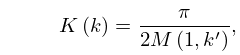
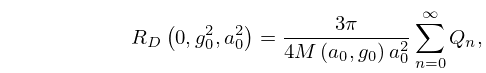
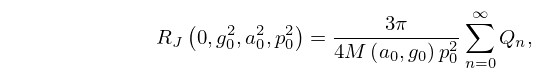
Finally, on taking the principal square roots of $k^{2}$ and ${k^{\prime}}^{2}$ we obtain values for $k$ and $k^{\prime}$ that lie in the 1st and 4th quadrants, respectively, and $2\omega_{1}$ , $2\omega_{3}$ are given by

23.22.1

2\omega_{1}M\left(1,k^{\prime}\right)=-2i\omega_{3}M\left(1,k\right)=\frac{\pi% }{3}\sqrt{\frac{c(2+k^{2}{k^{\prime}}^{2})({k^{\prime}}^{2}-k^{2})}{d(1-k^{2}{% k^{\prime}}^{2})}},

ⓘ

Symbols:: $M\left(\NVar{a},\NVar{g}\right)$ : arithmetic-geometric mean, $\pi$ : the ratio of the circumference of a circle to its diameter, $\mathrm{i}$ : imaginary unit, $\omega_{1}$ , $\omega_{3}$ , $\omega_{2}=-\omega_{1}-\omega_{3}$ : lattice generators, $k$ : modulus and $k^{\prime}$ : complementary modulus
Proof sketch:: Combine (23.6.16), (23.6.17), (22.20.6), (23.3.5)–(23.3.7), and use analytical continuation.
Referenced by:: §23.22(ii)
Permalink:: http://dlmf.nist.gov/23.22.E1
Encodings:: pMML, png, TeX
See also:: Annotations for §23.22(ii), §23.22(ii), §23.22 and Ch.23

where $M$ denotes the arithmetic-geometric mean (see §§19.8(i) and 22.20(ii)). This process yields 2 possible pairs ( $2\omega_{1}$ , $2\omega_{3}$ ), corresponding to the 2 possible choices of the square root.

…

6: Bibliography C

… ►

D. A. Cox (1984) The arithmetic-geometric mean of Gauss. Enseign. Math. (2) 30 (3-4), pp. 275–330.

ⓘ

External Links:: ISSN 0013-8584, MathReview (Bruce C. Berndt), ZentralBlatt
Referenced by:: §19.8(i).
Encodings:: BibTeX

►

D. A. Cox (1985) Gauss and the arithmetic-geometric mean. Notices Amer. Math. Soc. 32 (2), pp. 147–151.

ⓘ

External Links:: ISSN 0002-9920, MathReview (Willard Parker)
Referenced by:: §19.8(i).
Encodings:: BibTeX

…

7: Bibliography

… ►

G. Almkvist and B. Berndt (1988) Gauss, Landen, Ramanujan, the arithmetic-geometric mean, ellipses,

\pi

, and the Ladies Diary. Amer. Math. Monthly 95 (7), pp. 585–608.

ⓘ

External Links:: ISSN 0002-9890, FullText, Document, MathReview (R. A. Askey), ZentralBlatt
Referenced by:: §19.9(i).
Encodings:: BibTeX

…

8: Bibliography S

… ►

K. L. Sala (1989) Transformations of the Jacobian amplitude function and its calculation via the arithmetic-geometric mean. SIAM J. Math. Anal. 20 (6), pp. 1514–1528.

ⓘ

External Links:: ISSN 0036-1410, Document, MathReview (J. M. H. Peters), ZentralBlatt
Referenced by:: §22.19(i), §22.20(vi).
Encodings:: BibTeX

…

9: 15.8 Transformations of Variable

… ►This is used in a cubic analog of the arithmetic-geometric mean. …