apetamin p pills cheaP-pHarma.com/?id=1738

Did you mean upeta p mills cheema-parma/?id=1738 ?

(0.052 seconds)

1—10 of 538 matching pages

2: 27.9 Quadratic Characters

… ►If

p

divides

n

, then the value of

(n|p)

0

. …It is sometimes written as

(\frac{n}{p})

. … ►If

p, q

are distinct odd primes, then the quadratic reciprocity law states that … ►The Jacobi symbol

(n|P)

is a Dirichlet character (mod

P

). Both (27.9.1) and (27.9.2) are valid with

p

replaced by

P

; the reciprocity law (27.9.3) holds if

p, q

are replaced by any two relatively prime odd integers

P, Q

3: 29.15 Fourier Series and Chebyshev Series

… ►be the tridiagonal matrix with

\alpha_{p}

\beta_{p}

\gamma_{p}

as in (29.3.11), (29.3.12). … ►In (29.15.2) replace

\alpha_{p}

\beta_{p}

, and

\gamma_{p}

as in (29.3.13), (29.3.14). … ►In (29.15.2) replace

\alpha_{p}

\beta_{p}

, and

\gamma_{p}

as in (29.3.15), (29.3.16). … ►In (29.15.2) replace

\alpha_{p}

\beta_{p}

, and

\gamma_{p}

as in (29.6.11). … ►In (29.15.2) replace

\alpha_{p}

\beta_{p}

, and

\gamma_{p}

as in (29.3.17). …

6: 24.10 Arithmetic Properties

… ►Here and elsewhere in §24.10 the symbol

p

denotes a prime number. …where the summation is over all

p

such that

p-1

divides

2n

. The denominator of

B_{2n}

is the product of all these primes

p

. … ►valid when

m\equiv n\pmod{(p-1)p^{\ell}}

and

n\not\equiv 0\pmod{p-1}

, where

\ell(\geq 0)

is a fixed integer. …where

p(>2)

is a prime and

n\geq 2

. …

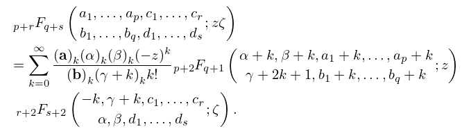
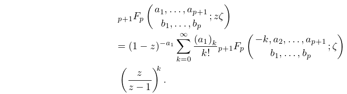
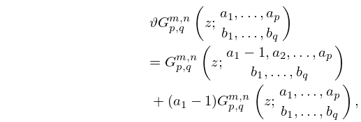
7: 16.10 Expansions in Series of ${{}_{p}F_{q}}$ Functions

§16.10 Expansions in Series of ${{}_{p}F_{q}}$ Functions

… ►

16.10.1

{{}_{p+r}F_{q+s}}\left({a_{1},\dots,a_{p},c_{1},\dots,c_{r}\atop b_{1},\dots,b% _{q},d_{1},\dots,d_{s}};z\zeta\right)=\sum_{k=0}^{\infty}\frac{{\left(\mathbf{% a}\right)_{k}}{\left(\alpha\right)_{k}}{\left(\beta\right)_{k}}(-z)^{k}}{{% \left(\mathbf{b}\right)_{k}}{\left(\gamma+k\right)_{k}}k!}{{}_{p+2}F_{q+1}}% \left({\alpha+k,\beta+k,a_{1}+k,\dots,a_{p}+k\atop\gamma+2k+1,b_{1}+k,\dots,b_% {q}+k};z\right){{}_{r+2}F_{s+2}}\left({-k,\gamma+k,c_{1},\dots,c_{r}\atop% \alpha,\beta,d_{1},\dots,d_{s}};\zeta\right).

ⓘ

Symbols:: ${{}_{\NVar{p}}F_{\NVar{q}}}\left(\NVar{a_{1},\dots,a_{p}};\NVar{b_{1},\dots,b_% {q}};\NVar{z}\right)$ or ${{}_{\NVar{p}}F_{\NVar{q}}}\left({\NVar{a_{1},\dots,a_{p}}\atop\NVar{b_{1},% \dots,b_{q}}};\NVar{z}\right)$ : alternatively ${{}_{\NVar{p}}F_{\NVar{q}}}\left(\NVar{\mathbf{a}};\NVar{\mathbf{b}};\NVar{z}\right)$ or ${{}_{\NVar{p}}F_{\NVar{q}}}\left({\NVar{\mathbf{a}}\atop\NVar{\mathbf{b}}};% \NVar{z}\right)$
generalized hypergeometric function, ${\left(\NVar{a}\right)_{\NVar{n}}}$ : Pochhammer’s symbol (or shifted factorial), $!$ : factorial (as in $n!$ ), $p$ : nonnegative integer, $q$ : nonnegative integer, $z$ : complex variable, $a,a_{1},\ldots,a_{p}$ : real or complex parameters and $b,b_{1},\ldots,b_{q}$ : real or complex parameters
Permalink:: http://dlmf.nist.gov/16.10.E1
Encodings:: pMML, png, TeX
See also:: Annotations for §16.10 and Ch.16

… ►

16.10.2

{{}_{p+1}F_{p}}\left({a_{1},\dots,a_{p+1}\atop b_{1},\dots,b_{p}};z\zeta\right% )=(1-z)^{-a_{1}}\sum_{k=0}^{\infty}\frac{{\left(a_{1}\right)_{k}}}{k!}{{}_{p+1% }F_{p}}\left({-k,a_{2},\dots,a_{p+1}\atop b_{1},\dots,b_{p}};\zeta\right)\left% (\frac{z}{z-1}\right)^{k}.

ⓘ

Symbols:: ${{}_{\NVar{p}}F_{\NVar{q}}}\left(\NVar{a_{1},\dots,a_{p}};\NVar{b_{1},\dots,b_% {q}};\NVar{z}\right)$ or ${{}_{\NVar{p}}F_{\NVar{q}}}\left({\NVar{a_{1},\dots,a_{p}}\atop\NVar{b_{1},% \dots,b_{q}}};\NVar{z}\right)$ : alternatively ${{}_{\NVar{p}}F_{\NVar{q}}}\left(\NVar{\mathbf{a}};\NVar{\mathbf{b}};\NVar{z}\right)$ or ${{}_{\NVar{p}}F_{\NVar{q}}}\left({\NVar{\mathbf{a}}\atop\NVar{\mathbf{b}}};% \NVar{z}\right)$
generalized hypergeometric function, ${\left(\NVar{a}\right)_{\NVar{n}}}$ : Pochhammer’s symbol (or shifted factorial), $!$ : factorial (as in $n!$ ), $p$ : nonnegative integer, $z$ : complex variable, $a,a_{1},\ldots,a_{p}$ : real or complex parameters and $b,b_{1},\ldots,b_{q}$ : real or complex parameters
Permalink:: http://dlmf.nist.gov/16.10.E2
Encodings:: pMML, png, TeX
See also:: Annotations for §16.10 and Ch.16

… ►Expansions of the form

\sum_{n=1}^{\infty}(\pm 1)^{n}{{}_{p}F_{p+1}}\left(\mathbf{a};\mathbf{b};-n^{2% }z^{2}\right)

are discussed in Miller (1997), and further series of generalized hypergeometric functions are given in Luke (1969b, Chapter 9), Luke (1975, §§5.10.2 and 5.11), and Prudnikov et al. (1990, §§5.3, 6.8–6.9).

8: 32.1 Special Notation

… ►The functions treated in this chapter are the solutions of the Painlevé equations

\mbox{P}_{\mbox{\scriptsize I}}

–

\mbox{P}_{\mbox{\scriptsize VI}}

9: 16.19 Identities

… ►

16.19.1

{G^{m,n}_{p,q}}\left(\frac{1}{z};{a_{1},\dots,a_{p}\atop b_{1},\dots,b_{q}}% \right)={G^{n,m}_{q,p}}\left(z;{1-b_{1},\dots,1-b_{q}\atop 1-a_{1},\dots,1-a_{% p}}\right),

ⓘ

Symbols:: ${G^{\NVar{m},\NVar{n}}_{\NVar{p},\NVar{q}}}\left(\NVar{z};{\NVar{a_{1},\dots,a% _{p}}\atop\NVar{b_{1},\dots,b_{q}}}\right)$ or ${G^{\NVar{m},\NVar{n}}_{\NVar{p},\NVar{q}}}\left(\NVar{z};\NVar{\mathbf{a}};% \NVar{\mathbf{b}}\right)$ : Meijer $G$ -function, $p$ : nonnegative integer, $q$ : nonnegative integer, $z$ : complex variable, $a,a_{1},\ldots,a_{p}$ : real or complex parameters and $b,b_{1},\ldots,b_{q}$ : real or complex parameters
Referenced by:: §16.21
Permalink:: http://dlmf.nist.gov/16.19.E1
Encodings:: pMML, png, TeX
See also:: Annotations for §16.19 and Ch.16

►

16.19.2

z^{\mu}{G^{m,n}_{p,q}}\left(z;{a_{1},\dots,a_{p}\atop b_{1},\dots,b_{q}}\right% )={G^{m,n}_{p,q}}\left(z;{a_{1}+\mu,\dots,a_{p}+\mu\atop b_{1}+\mu,\dots,b_{q}% +\mu}\right),

ⓘ

Symbols:: ${G^{\NVar{m},\NVar{n}}_{\NVar{p},\NVar{q}}}\left(\NVar{z};{\NVar{a_{1},\dots,a% _{p}}\atop\NVar{b_{1},\dots,b_{q}}}\right)$ or ${G^{\NVar{m},\NVar{n}}_{\NVar{p},\NVar{q}}}\left(\NVar{z};\NVar{\mathbf{a}};% \NVar{\mathbf{b}}\right)$ : Meijer $G$ -function, $p$ : nonnegative integer, $q$ : nonnegative integer, $z$ : complex variable, $a,a_{1},\ldots,a_{p}$ : real or complex parameters and $b,b_{1},\ldots,b_{q}$ : real or complex parameters
Permalink:: http://dlmf.nist.gov/16.19.E2
Encodings:: pMML, png, TeX
See also:: Annotations for §16.19 and Ch.16

►

16.19.3

{G^{m,n+1}_{p+1,q+1}}\left(z;{a_{0},\dots,a_{p}\atop b_{1},\dots,b_{q},a_{0}}% \right)={G^{m,n}_{p,q}}\left(z;{a_{1},\dots,a_{p}\atop b_{1},\dots,b_{q}}% \right),

ⓘ

Symbols:: ${G^{\NVar{m},\NVar{n}}_{\NVar{p},\NVar{q}}}\left(\NVar{z};{\NVar{a_{1},\dots,a% _{p}}\atop\NVar{b_{1},\dots,b_{q}}}\right)$ or ${G^{\NVar{m},\NVar{n}}_{\NVar{p},\NVar{q}}}\left(\NVar{z};\NVar{\mathbf{a}};% \NVar{\mathbf{b}}\right)$ : Meijer $G$ -function, $p$ : nonnegative integer, $q$ : nonnegative integer, $z$ : complex variable, $a,a_{1},\ldots,a_{p}$ : real or complex parameters and $b,b_{1},\ldots,b_{q}$ : real or complex parameters
Permalink:: http://dlmf.nist.gov/16.19.E3
Encodings:: pMML, png, TeX
See also:: Annotations for §16.19 and Ch.16

►

16.19.4

{G^{m,n}_{p,q}}\left(z;{a_{1},\dots,a_{p}\atop b_{1},\dots,b_{q}}\right)=\frac% {2^{p+1+b_{1}+\dots+b_{q}-m-n-a_{1}-\dots-a_{p}}}{\pi^{m+n-\frac{1}{2}(p+q)}}{% G^{2m,2n}_{2p,2q}}\left(2^{2p-2q}z^{2};{\frac{1}{2}a_{1},\frac{1}{2}a_{1}+% \frac{1}{2},\dots,\frac{1}{2}a_{p},\frac{1}{2}a_{p}+\frac{1}{2}\atop\frac{1}{2% }b_{1},\frac{1}{2}b_{1}+\frac{1}{2},\dots,\frac{1}{2}b_{q},\frac{1}{2}b_{q}+% \frac{1}{2}}\right),

ⓘ

Symbols:: ${G^{\NVar{m},\NVar{n}}_{\NVar{p},\NVar{q}}}\left(\NVar{z};{\NVar{a_{1},\dots,a% _{p}}\atop\NVar{b_{1},\dots,b_{q}}}\right)$ or ${G^{\NVar{m},\NVar{n}}_{\NVar{p},\NVar{q}}}\left(\NVar{z};\NVar{\mathbf{a}};% \NVar{\mathbf{b}}\right)$ : Meijer $G$ -function, $\pi$ : the ratio of the circumference of a circle to its diameter, $p$ : nonnegative integer, $q$ : nonnegative integer, $z$ : complex variable, $a,a_{1},\ldots,a_{p}$ : real or complex parameters and $b,b_{1},\ldots,b_{q}$ : real or complex parameters
Permalink:: http://dlmf.nist.gov/16.19.E4
Encodings:: pMML, png, TeX
See also:: Annotations for §16.19 and Ch.16

►

16.19.5

\vartheta{G^{m,n}_{p,q}}\left(z;{a_{1},\dots,a_{p}\atop b_{1},\dots,b_{q}}% \right)={G^{m,n}_{p,q}}\left(z;{a_{1}-1,a_{2},\dots,a_{p}\atop b_{1},\dots,b_{% q}}\right)+(a_{1}-1){G^{m,n}_{p,q}}\left(z;{a_{1},\dots,a_{p}\atop b_{1},\dots% ,b_{q}}\right),

ⓘ

Symbols:: ${G^{\NVar{m},\NVar{n}}_{\NVar{p},\NVar{q}}}\left(\NVar{z};{\NVar{a_{1},\dots,a% _{p}}\atop\NVar{b_{1},\dots,b_{q}}}\right)$ or ${G^{\NVar{m},\NVar{n}}_{\NVar{p},\NVar{q}}}\left(\NVar{z};\NVar{\mathbf{a}};% \NVar{\mathbf{b}}\right)$ : Meijer $G$ -function, $p$ : nonnegative integer, $q$ : nonnegative integer, $z$ : complex variable, $a,a_{1},\ldots,a_{p}$ : real or complex parameters, $b,b_{1},\ldots,b_{q}$ : real or complex parameters and $\vartheta$ : differential operator
Permalink:: http://dlmf.nist.gov/16.19.E5
Encodings:: pMML, png, TeX
See also:: Annotations for §16.19 and Ch.16

…

10: 29.7 Asymptotic Expansions

… ►

p=2m+1,

… ►

29.7.4

\tau_{1}=\frac{p}{2^{6}}((1+k^{2})^{2}(p^{2}+3)-4k^{2}(p^{2}+5)).

ⓘ

Symbols:: $p$ : nonnegative integer, $k$ : real parameter and $\tau_{j}$ : coefficients
Permalink:: http://dlmf.nist.gov/29.7.E4
Encodings:: pMML, png, TeX
See also:: Annotations for §29.7(i), §29.7 and Ch.29

… ►

29.7.6

\tau_{2}=\frac{1}{2^{10}}(1+k^{2})(1-k^{2})^{2}(5p^{4}+34p^{2}+9),

ⓘ

Symbols:: $p$ : nonnegative integer, $k$ : real parameter and $\tau_{j}$ : coefficients
Permalink:: http://dlmf.nist.gov/29.7.E6
Encodings:: pMML, png, TeX
See also:: Annotations for §29.7(i), §29.7 and Ch.29

►

29.7.7

\tau_{3}=\frac{p}{2^{14}}((1+k^{2})^{4}(33p^{4}+410p^{2}+405)-24k^{2}(1+k^{2})% ^{2}(7p^{4}+90p^{2}+95)+16k^{4}(9p^{4}+130p^{2}+173)),

ⓘ

Symbols:: $p$ : nonnegative integer, $k$ : real parameter and $\tau_{j}$ : coefficients
Permalink:: http://dlmf.nist.gov/29.7.E7
Encodings:: pMML, png, TeX
See also:: Annotations for §29.7(i), §29.7 and Ch.29

►

29.7.8

\tau_{4}=\frac{1}{2^{16}}((1+k^{2})^{5}(63p^{6}+1260p^{4}+2943p^{2}+486)-8k^{2% }(1+k^{2})^{3}(49p^{6}+1010p^{4}+2493p^{2}+432)+16k^{4}(1+k^{2})(35p^{6}+760p^% {4}+2043p^{2}+378)).

ⓘ

Symbols:: $p$ : nonnegative integer, $k$ : real parameter and $\tau_{j}$ : coefficients
Permalink:: http://dlmf.nist.gov/29.7.E8
Encodings:: pMML, png, TeX
See also:: Annotations for §29.7(i), §29.7 and Ch.29

…

apetamin p pills cheaP-pHarma.com/?id=1738

1—10 of 538 matching pages

1: 29.6 Fourier Series

2: 27.9 Quadratic Characters

3: 29.15 Fourier Series and Chebyshev Series

4: 16.9 Zeros

5: 20 Theta Functions

6: 24.10 Arithmetic Properties

7: 16.10 Expansions in Series of ${{}_{p}F_{q}}$ Functions

§16.10 Expansions in Series of ${{}_{p}F_{q}}$ Functions

8: 32.1 Special Notation

9: 16.19 Identities

10: 29.7 Asymptotic Expansions

apetamin p pills cheaP-pHarma.com/?id=1738

1—10 of 538 matching pages

1: 29.6 Fourier Series

2: 27.9 Quadratic Characters

3: 29.15 Fourier Series and Chebyshev Series

4: 16.9 Zeros

5: 20 Theta Functions

6: 24.10 Arithmetic Properties

7: 16.10 Expansions in Series of F q p Functions

§16.10 Expansions in Series of F q p Functions

8: 32.1 Special Notation

9: 16.19 Identities

10: 29.7 Asymptotic Expansions

7: 16.10 Expansions in Series of ${{}_{p}F_{q}}$ Functions

§16.10 Expansions in Series of ${{}_{p}F_{q}}$ Functions