Verblunsky theorem

SearchAdvancedHelp

(0.001 seconds)

1—10 of 120 matching pages

1: 18.33 Polynomials Orthogonal on the Unit Circle

… ►

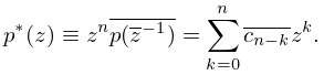
18.33.22 $$p^{\ast }(z)\equiv z^n\overline{p({\overline{z}}^{-1})}=\sum _{k=0}^n\overline{c_{n-k}}{z}^k.$$

ⓘ

Symbols:

$\overline{z}$: complex conjugate, $\equiv$: equals by definition, $z$: complex variable, $k$: nonnegative integer and $n$: nonnegative integer

Source:

Simon (2005a, (1.1.7))

Permalink:

http://dlmf.nist.gov/18.33.E22

Encodings:

pMML, png, TeX

See also:

Annotations for §18.33(vi), §18.33(vi), §18.33 and Ch.18

►The Verblunsky coefficients (also called Schur parameters or reflection coefficients) are the coefficients ${\alpha }_n$ in the Szegő recurrence relations … ►

Verblunsky’s Theorem

… ►

Szegő’s Theorem

►For $w(z)$ as in (18.33.19) (or more generally as the weight function of the absolutely continuous part of the measure $\mu$ in (18.33.17)) and with ${\alpha }_n$ the Verblunsky coefficients in (18.33.23), (18.33.24), Szegő’s theorem states that …

2: 28.27 Addition Theorems

§28.27 Addition Theorems

►Addition theorems provide important connections between Mathieu functions with different parameters and in different coordinate systems. They are analogous to the addition theorems for Bessel functions (§10.23(ii)) and modified Bessel functions (§10.44(ii)). …

3: 27.15 Chinese Remainder Theorem

§27.15 Chinese Remainder Theorem

►The Chinese remainder theorem states that a system of congruences $x\equiv a_1(mod{m}_1),\mathrm{\dots },x\equiv a_k(mod{m}_k)$, always has a solution if the moduli are relatively prime in pairs; the solution is unique (mod $m$), where $m$ is the product of the moduli. ►This theorem is employed to increase efficiency in calculating with large numbers by making use of smaller numbers in most of the calculation. …By the Chinese remainder theorem each integer in the data can be uniquely represented by its residues (mod $m_1$), (mod $m_2$), (mod $m_3$), and (mod $m_4$), respectively. …These numbers, in turn, are combined by the Chinese remainder theorem to obtain the final result $(modm)$, which is correct to 20 digits. …

4: 30.10 Series and Integrals

… ►For an addition theorem, see Meixner and Schäfke (1954, p. 300) and King and Van Buren (1973). …

5: 10.44 Sums

… ►

§10.44(i) Multiplication Theorem

… ►

§10.44(ii) Addition Theorems

►

Neumann’s Addition Theorem

… ►

Graf’s and Gegenbauer’s Addition Theorems

…

6: 19.35 Other Applications

… ►

§19.35(i) Mathematical

►Generalizations of elliptic integrals appear in analysis of modular theorems of Ramanujan (Anderson et al. (2000)); analysis of Selberg integrals (Van Diejen and Spiridonov (2001)); use of Legendre’s relation (19.7.1) to compute $\pi$ to high precision (Borwein and Borwein (1987, p. 26)). …

7: 13.13 Addition and Multiplication Theorems

§13.13 Addition and Multiplication Theorems

►

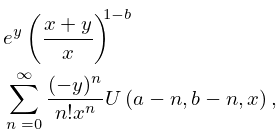
§13.13(i) Addition Theorems for $M(a,b,z)$

… ►

§13.13(ii) Addition Theorems for $U(a,b,z)$

… ►

13.13.12 $${\mathrm{e}}^y{\left(\frac{x+y}{x}\right)}^{1-b}\sum _{n=0}^{\mathrm{\infty }}\frac{{(-y)}^n}{n!x^n}U(a-n,b-n,x),$$ .

ⓘ

Symbols:

$U(a,b,z)$: Kummer confluent hypergeometric function, $\mathrm{e}$: base of natural logarithm, $!$: factorial (as in $n!$), $n$: nonnegative integer, $x$: real variable and $y$: real variable

Permalink:

http://dlmf.nist.gov/13.13.E12

Encodings:

pMML, png, TeX

See also:

Annotations for §13.13(ii), §13.13 and Ch.13

►

§13.13(iii) Multiplication Theorems for $M(a,b,z)$ and $U(a,b,z)$

…

8: 10.23 Sums

… ►

§10.23(i) Multiplication Theorem

… ►

§10.23(ii) Addition Theorems

►

Neumann’s Addition Theorem

… ►

Graf’s and Gegenbauer’s Addition Theorems

… ► …

9: 27.16 Cryptography

… ►Thus, $y\equiv x^r(modn)$ and . … ►By the Euler–Fermat theorem (27.2.8), $x^{\varphi \left(n\right)}\equiv 1(modn)$; hence $x^{t\varphi \left(n\right)}\equiv 1(modn)$. …

10: 14.28 Sums

… ►

§14.28(i) Addition Theorem

… ►For generalizations in terms of Gegenbauer and Jacobi polynomials, see Theorem 2. 1 in Cohl (2013b) and Theorem 1 in Cohl (2013a) respectively. …