Riemann

SearchAdvancedHelp

(0.001 seconds)

11—20 of 91 matching pages

11: 8.22 Mathematical Applications

… ►

§8.22(ii) Riemann Zeta Function and Incomplete Riemann Zeta Function

… ►See Paris and Cang (1997). ►If ${\zeta }_x(s)$ denotes the incomplete Riemann zeta function defined by …so that ${lim}_{x\to \mathrm{\infty }}{\zeta }_x(s)=\zeta \left(s\right)$, then …For further information on ${\zeta }_x(s)$, including zeros and uniform asymptotic approximations, see Kölbig (1970, 1972a) and Dunster (2006). …

12: 25.4 Reflection Formulas

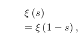
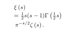
§25.4 Reflection Formulas

… ►

25.4.1 $$\zeta \left(1-s\right)=2{(2\pi )}^{-s}\cos \left(\frac{1}{2}\pi s\right)\mathrm{\Gamma }\left(s\right)\zeta \left(s\right),$$

ⓘ

Symbols:

$\mathrm{\Gamma }\left(z\right)$: gamma function, $\zeta \left(s\right)$: Riemann zeta function, $\pi$: the ratio of the circumference of a circle to its diameter, $\cos z$: cosine function and $s$: complex variable

Keywords:

reflection formula

Source:

Apostol (1976, (12), p. 259)

Referenced by:

§25.10(i), §5.17

Permalink:

http://dlmf.nist.gov/25.4.E1

Encodings:

pMML, png, TeX

See also:

Annotations for §25.4 and Ch.25

… ►

25.4.3 $$\xi \left(s\right)=\xi \left(1-s\right),$$

ⓘ

Symbols:

$\xi \left(s\right)$: Riemann’s $\xi$-function and $s$: complex variable

Keywords:

reflection formula

Source:

Apostol (1976, p. 260)

Permalink:

http://dlmf.nist.gov/25.4.E3

Encodings:

pMML, png, TeX

See also:

Annotations for §25.4 and Ch.25

►where $\xi \left(s\right)$ is Riemann’s $\xi$-function, defined by: ►

25.4.4 $$\xi \left(s\right)=\frac{1}{2}s(s-1)\mathrm{\Gamma }\left(\frac{1}{2}s\right){\pi }^{-s/2}\zeta \left(s\right).$$

ⓘ

Defines:

$\xi \left(s\right)$: Riemann’s $\xi$-function

Symbols:

$\mathrm{\Gamma }\left(z\right)$: gamma function, $\zeta \left(s\right)$: Riemann zeta function, $\pi$: the ratio of the circumference of a circle to its diameter and $s$: complex variable

Keywords:

definition

Source:

Apostol (1976, p. 260)

Permalink:

http://dlmf.nist.gov/25.4.E4

Encodings:

pMML, png, TeX

See also:

Annotations for §25.4 and Ch.25

…

13: 25.3 Graphics

§25.3 Graphics

►

►►

Figure 25.3.1: Riemann zeta function $\zeta \left(x\right)$ and its derivative ${\zeta }^{\prime }\left(x\right)$, $-20\le x\le 10$. Magnify

►

►►

Figure 25.3.2: Riemann zeta function $\zeta \left(x\right)$ and its derivative ${\zeta }^{\prime }\left(x\right)$, $-12\le x\le -2$. Magnify

… ►

►►

Figure 25.3.4: $Z(t)$, $0\le t\le 50$. $Z(t)$ and $\zeta \left(\frac{1}{2}+\mathrm{i}t\right)$ have the same zeros. … Magnify

… ►

►►

Figure 25.3.6: $Z(t)$, $10000\le t\le 10050$. Magnify

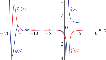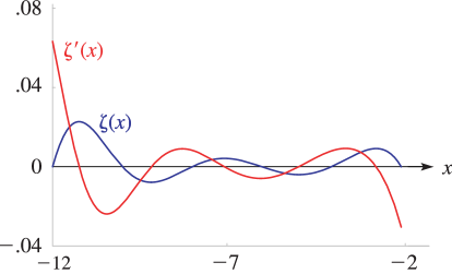14: 25.18 Methods of Computation

… ►

§25.18(i) Function Values and Derivatives

►The principal tools for computing $\zeta \left(s\right)$ are the expansion (25.2.9) for general values of $s$, and the Riemann–Siegel formula (25.10.3) (extended to higher terms) for $\zeta \left(\frac{1}{2}+\mathrm{i}t\right)$. …Calculations relating to derivatives of $\zeta \left(s\right)$ and/or $\zeta (s,a)$ can be found in Apostol (1985a), Choudhury (1995), Miller and Adamchik (1998), and Yeremin et al. (1988). … ►

§25.18(ii) Zeros

►Most numerical calculations of the Riemann zeta function are concerned with locating zeros of $\zeta \left(\frac{1}{2}+\mathrm{i}t\right)$ in an effort to prove or disprove the Riemann hypothesis, which states that all nontrivial zeros of $\zeta \left(s\right)$ lie on the critical line $\mathrm{\Re }s=\frac{1}{2}$. …

15: 21.4 Graphics

§21.4 Graphics

►Figure 21.4.1 provides surfaces of the scaled Riemann theta function $\widehat{\theta }\left(𝐳\right|𝛀)$, with …This Riemann matrix originates from the Riemann surface represented by the algebraic curve ${\mu }^3-{\lambda }^7+2{\lambda }^3\mu =0$; compare §21.7(i). … ►For the scaled Riemann theta functions depicted in Figures 21.4.2–21.4.5 … ►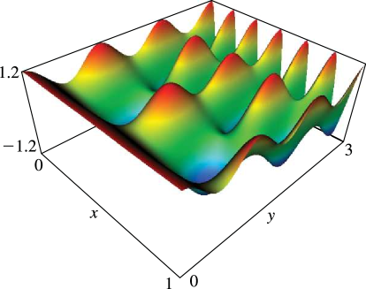

►

►

Figure 21.4.5: The real part of a genus 3 scaled Riemann theta function: $\mathrm{\Re }\widehat{\theta }\left(x+\mathrm{i}y,0,0\right|{𝛀}_2)$, $0\le x\le 1$, $0\le y\le 3$. … Magnify 3D Help

16: 25.10 Zeros

… ►

§25.10(i) Distribution

… ►The Riemann hypothesis states that all nontrivial zeros lie on this line. … ►

§25.10(ii) Riemann–Siegel Formula

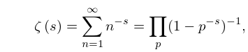
… ►Riemann also developed a technique for determining further terms. …

17: 27.4 Euler Products and Dirichlet Series

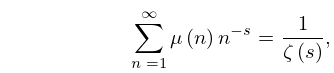
… ►The completely multiplicative function $f(n)=n^{-s}$ gives the Euler product representation of the Riemann zeta function $\zeta \left(s\right)$ (§25.2(i)): ►

27.4.3 $$\zeta \left(s\right)=\sum _{n=1}^{\mathrm{\infty }}{n}^{-s}=\prod _p{(1-p^{-s})}^{-1},$$ $\mathrm{\Re }s>1$.

ⓘ

Symbols:

$\zeta \left(s\right)$: Riemann zeta function, $\mathrm{\Re }$: real part, $n$: positive integer and $p,p_1,\mathrm{\dots }$: prime numbers

A&S Ref:

23.2.1 and 23.2.2

Permalink:

http://dlmf.nist.gov/27.4.E3

Encodings:

pMML, png, TeX

See also:

Annotations for §27.4 and Ch.27

►The Riemann zeta function is the prototype of series of the form … ►

27.4.5 $$\sum _{n=1}^{\mathrm{\infty }}\mu \left(n\right)n^{-s}=\frac{1}{\zeta \left(s\right)},$$ $\mathrm{\Re }s>1$,

ⓘ

Symbols:

$\mu \left(n\right)$: Möbius function, $\zeta \left(s\right)$: Riemann zeta function, $\mathrm{\Re }$: real part and $n$: positive integer

A&S Ref:

24.3.1 I.B

Permalink:

http://dlmf.nist.gov/27.4.E5

Encodings:

pMML, png, TeX

See also:

Annotations for §27.4 and Ch.27

… ►In (27.4.12) and (27.4.13) ${\zeta }^{\prime }\left(s\right)$ is the derivative of $\zeta \left(s\right)$.

18: 25.6 Integer Arguments

… ►

§25.6(i) Function Values

… ►

25.6.4 $$\zeta \left(-2n\right)=0,$$ $n=1,2,3,\mathrm{\dots }$.

ⓘ

Symbols:

$\zeta \left(s\right)$: Riemann zeta function and $n$: nonnegative integer

Source:

Apostol (1976, Theorem 12.16, p. 266)

A&S Ref:

23.2.14

Permalink:

http://dlmf.nist.gov/25.6.E4

Encodings:

pMML, png, TeX

See also:

Annotations for §25.6(i), §25.6 and Ch.25

… ►

§25.6(ii) Derivative Values

… ►

§25.6(iii) Recursion Formulas

►

25.6.16 $$\left(n+\frac{1}{2}\right)\zeta \left(2n\right)=\sum _{k=1}^{n-1}\zeta \left(2k\right)\zeta \left(2n-2k\right),$$ $n\ge 2$.

ⓘ

Symbols:

$\zeta \left(s\right)$: Riemann zeta function, $k$: nonnegative integer and $n$: nonnegative integer

Source:

Basu and Apostol (2000, (1.5), p. 397)

Permalink:

http://dlmf.nist.gov/25.6.E16

Encodings:

pMML, png, TeX

See also:

Annotations for §25.6(iii), §25.6 and Ch.25

…

19: 21.5 Modular Transformations

… ►

§21.5(i) Riemann Theta Functions

… ►Equation (21.5.4) is the modular transformation property for Riemann theta functions. ►The modular transformations form a group under the composition of such transformations, the modular group, which is generated by simpler transformations, for which $\xi (𝚪)$ is determinate: … ►

§21.5(ii) Riemann Theta Functions with Characteristics

… ►For explicit results in the case $g=1$, see §20.7(viii).

20: 25.8 Sums

§25.8 Sums

►

25.8.1 $$\sum _{k=2}^{\mathrm{\infty }}\left(\zeta \left(k\right)-1\right)=1.$$

ⓘ

Symbols:

$\zeta \left(s\right)$: Riemann zeta function and $k$: nonnegative integer

Keywords:

infinite series

Source:

Adamchik and Srivastava (1998, (1.4), p. 132)

Permalink:

http://dlmf.nist.gov/25.8.E1

Encodings:

pMML, png, TeX

See also:

Annotations for §25.8 and Ch.25

►

25.8.2 $$\sum _{k=0}^{\mathrm{\infty }}\frac{\mathrm{\Gamma }\left(s+k\right)}{(k+1)!}\left(\zeta \left(s+k\right)-1\right)=\mathrm{\Gamma }\left(s-1\right),$$ $s\ne 1,0,-1,-2,\mathrm{\dots }$.

ⓘ

Symbols:

$\mathrm{\Gamma }\left(z\right)$: gamma function, $\zeta \left(s\right)$: Riemann zeta function, $!$: factorial (as in $n!$), $k$: nonnegative integer and $s$: complex variable

Keywords:

infinite series

Source:

Landau (1953, (2), p. 273); with (5.2.4), (5.2.5)

Permalink:

http://dlmf.nist.gov/25.8.E2

Encodings:

pMML, png, TeX

See also:

Annotations for §25.8 and Ch.25

… ►

25.8.9 $$\sum _{k=1}^{\mathrm{\infty }}\frac{\zeta \left(2k\right)}{(2k+1)2^{2k}}=\frac{1}{2}-\frac{1}{2}\ln 2.$$

ⓘ

Symbols:

$\zeta \left(s\right)$: Riemann zeta function, $\ln z$: principal branch of logarithm function and $k$: nonnegative integer

Keywords:

infinite series

Source:

Srivastava and Choi (2001, (467), p. 212)

Permalink:

http://dlmf.nist.gov/25.8.E9

Encodings:

pMML, png, TeX

See also:

Annotations for §25.8 and Ch.25

►

25.8.10 $$\sum _{k=1}^{\mathrm{\infty }}\frac{\zeta \left(2k\right)}{(2k+1)(2k+2)2^{2k}}=\frac{1}{4}-\frac{7}{4{\pi }^2}\zeta \left(3\right).$$

ⓘ

Symbols:

$\zeta \left(s\right)$: Riemann zeta function, $\pi$: the ratio of the circumference of a circle to its diameter and $k$: nonnegative integer

Keywords:

infinite series

Source:

Ewell (1990, (1), p. 219)

Permalink:

http://dlmf.nist.gov/25.8.E10

Encodings:

pMML, png, TeX

See also:

Annotations for §25.8 and Ch.25

…