Pfaff--Saalschutz%20formula

SearchAdvancedHelp

(0.003 seconds)

11—20 of 307 matching pages

11: 36.4 Bifurcation Sets

… ►

§36.4(i) Formulas

… ► $K=2$, cusp bifurcation set: … ► $K=3$, swallowtail bifurcation set: … ►Elliptic umbilic bifurcation set (codimension three): for fixed $z$, the section of the bifurcation set is a three-cusped astroid … ►Hyperbolic umbilic bifurcation set (codimension three): …

12: 3.4 Differentiation

… ►

Two-Point Formula

… ►

Three-Point Formula

… ►

Four-Point Formula

… ►

Five-Point Formula

… ►

Six-Point Formula

…

13: 36.5 Stokes Sets

… ►

§36.5(ii) Cuspoids

… ►

36.5.4 $$80x^5-40x^4-55x^3+5x^2+20x-1=0,$$

ⓘ

Symbols:

$x$: real parameter

Permalink:

http://dlmf.nist.gov/36.5.E4

Encodings:

pMML, png, TeX

See also:

Annotations for §36.5(ii), §36.5(ii), §36.5 and Ch.36

… ►

36.5.7 $$X=\frac{9}{20}+20u^4-\frac{Y^2}{20u^2}+6u^2\mathrm{sign}\left(z\right),$$

ⓘ

Symbols:

$\mathrm{sign}x$: sign of, $z$: real parameter, $X$: scaled coordinate and $Y$: scaled coordinate

Permalink:

http://dlmf.nist.gov/36.5.E7

Encodings:

pMML, png, TeX

See also:

Annotations for §36.5(ii), §36.5(ii), §36.5 and Ch.36

… ►

§36.5(iii) Umbilics

…

14: Bibliography N

… ►

On simplified asymptotic formulas for a class of Mathieu functions. SIAM J. Math. Anal. 15 (6), pp. 1205–1213.

ⓘ

External Links:

ISSN 0036-1410, Document, MathReview (Harold Exton), ZentralBlatt

Referenced by:

§28.26(ii).

Encodings:

BibTeX

►

On a simplified asymptotic formula for the Mathieu function of the third kind. SIAM J. Math. Anal. 18 (6), pp. 1616–1629.

ⓘ

External Links:

ISSN 0036-1410, Document, MathReview (F. M. Arscott), ZentralBlatt

Referenced by:

§28.26(ii).

Encodings:

BibTeX

►

On an integral transform involving a class of Mathieu functions. SIAM J. Math. Anal. 20 (6), pp. 1500–1513.

ⓘ

External Links:

ISSN 0036-1410, Document, MathReview (K. C. Gupta), ZentralBlatt

Referenced by:

§28.26(ii).

Encodings:

BibTeX

… ►

Reduction and evaluation of elliptic integrals. Math. Comp. 20 (94), pp. 223–231.

ⓘ

External Links:

FullText, MathReview (I. A. Stegun), ZentralBlatt

Referenced by:

§19.37(iv).

Encodings:

BibTeX

… ►

A table of integrals of the error functions. J. Res. Nat. Bur. Standards Sect B. 73B, pp. 1–20.

ⓘ

Notes:

See for additions and corrections same journal, Sect. B 75, 149–163 (1975)

External Links:

MathReview, ZentralBlatt

Referenced by:

§7.14(iii), §7.21, §7.7(iii).

Encodings:

BibTeX

…

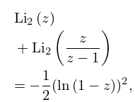
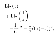
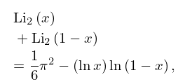
15: 25.12 Polylogarithms

… ►

25.12.3 $${\mathrm{Li}}_2\left(z\right)+{\mathrm{Li}}_2\left(\frac{z}{z-1}\right)=-\frac{1}{2}{(\ln \left(1-z\right))}^2,$$ $z\in ℂ\setminus [1,\mathrm{\infty })$.

ⓘ

Symbols:

$[a,b)$: half-closed interval, $ℂ$: complex plane, ${\mathrm{Li}}_2\left(z\right)$: dilogarithm, $\in$: element of, $\ln z$: principal branch of logarithm function, $\setminus$: set subtraction, $x$: real variable and $z$: complex variable

Keywords:

connection formula

Source:

Maximon (2003, (3.4), p. 2808)

A&S Ref:

27.7.5 (is a modified form with $z=1-x$)

Permalink:

http://dlmf.nist.gov/25.12.E3

Encodings:

pMML, png, TeX

See also:

Annotations for §25.12(i), §25.12 and Ch.25

►

25.12.4 $${\mathrm{Li}}_2\left(z\right)+{\mathrm{Li}}_2\left(\frac{1}{z}\right)=-\frac{1}{6}{\pi }^2-\frac{1}{2}{(\ln \left(-z\right))}^2,$$ $z\in ℂ\setminus [0,\mathrm{\infty })$.

ⓘ

Symbols:

$\pi$: the ratio of the circumference of a circle to its diameter, $[a,b)$: half-closed interval, $ℂ$: complex plane, ${\mathrm{Li}}_2\left(z\right)$: dilogarithm, $\in$: element of, $\ln z$: principal branch of logarithm function, $\setminus$: set subtraction and $z$: complex variable

Keywords:

connection formula

Source:

Maximon (2003, (3.2), p. 2808)

Referenced by:

§25.12(ii)

Permalink:

http://dlmf.nist.gov/25.12.E4

Encodings:

pMML, png, TeX

See also:

Annotations for §25.12(i), §25.12 and Ch.25

… ►

25.12.6 $${\mathrm{Li}}_2\left(x\right)+{\mathrm{Li}}_2\left(1-x\right)=\frac{1}{6}{\pi }^2-(\ln x)\ln \left(1-x\right),$$ .

ⓘ

Symbols:

$\pi$: the ratio of the circumference of a circle to its diameter, ${\mathrm{Li}}_2\left(z\right)$: dilogarithm, $\ln z$: principal branch of logarithm function and $x$: real variable

Keywords:

connection formula

Source:

Maximon (2003, (3.3), p. 2808)

Permalink:

http://dlmf.nist.gov/25.12.E6

Encodings:

pMML, png, TeX

See also:

Annotations for §25.12(i), §25.12 and Ch.25

… ►

►►

Figure 25.12.1: Dilogarithm function ${\mathrm{Li}}_2\left(x\right)$, Magnify

►

►

►

Figure 25.12.2: Absolute value of the dilogarithm function $\left|{\mathrm{Li}}_2\left(x+\mathrm{i}y\right)\right|$, $-20\le x\le 20$, $-20\le y\le 20$. … Magnify 3D Help

…

16: 17.4 Basic Hypergeometric Functions

… ►The series (17.4.1) is said to be balanced or Saalschützian when it terminates, $r=s$, $z=q$, and …

17: 28.35 Tables

… ►

Blanch and Clemm (1965) includes values of ${\mathrm{Mc}}_n^{(2)}(x,\sqrt{q})$, $\mathrm{Mc}_n^{(2)}{}_{}{}^{\prime }(x,\sqrt{q})$ for $n=0(1)7$, $x=0(.02)1$; $n=8(1)15$, $x=0(.01)1$. Also ${\mathrm{Ms}}_n^{(2)}(x,\sqrt{q})$, $\mathrm{Ms}_n^{(2)}{}_{}{}^{\prime }(x,\sqrt{q})$ for $n=1(1)7$, $x=0(.02)1$; $n=8(1)15$, $x=0(.01)1$. In all cases $q=0(.05)1$. Precision is generally 7D. Approximate formulas and graphs are also included.

… ►

Ince (1932) includes eigenvalues $a_n$, $b_n$, and Fourier coefficients for $n=0$ or $1(1)6$, $q=0(1)10(2)20(4)40$; 7D. Also ${\mathrm{ce}}_n(x,q)$, ${\mathrm{se}}_n(x,q)$ for $q=0(1)10$, $x=1(1)90$, corresponding to the eigenvalues in the tables; 5D. Notation: $a_n={\mathrm{𝑏𝑒}}_n-2q$, $b_n={\mathrm{𝑏𝑜}}_n-2q$.

►

Kirkpatrick (1960) contains tables of the modified functions ${\mathrm{Ce}}_n(x,q)$, ${\mathrm{Se}}_{n+1}(x,q)$ for $n=0(1)5$, $q=1(1)20$, $x=0.1(.1)1$; 4D or 5D.

►

National Bureau of Standards (1967) includes the eigenvalues $a_n\left(q\right)$, $b_n\left(q\right)$ for $n=0(1)3$ with $q=0(.2)20(.5)37(1)100$, and $n=4(1)15$ with $q=0(2)100$; Fourier coefficients for ${\mathrm{ce}}_n(x,q)$ and ${\mathrm{se}}_n(x,q)$ for $n=0(1)15$, $n=1(1)15$, respectively, and various values of $q$ in the interval $[0,100]$; joining factors $g_{e,n}(\sqrt{q})$, $f_{e,n}(\sqrt{q})$ for $n=0(1)15$ with $q=0(.5\text{ to }10)100$ (but in a different notation). Also, eigenvalues for large values of $q$. Precision is generally 8D.

… ►

Zhang and Jin (1996, pp. 521–532) includes the eigenvalues $a_n\left(q\right)$, $b_{n+1}\left(q\right)$ for $n=0(1)4$, $q=0(1)50$; $n=0(1)20$ ($a$’s) or 19 ($b$’s), $q=1,3,5,10,15,25,50(50)200$. Fourier coefficients for ${\mathrm{ce}}_n(x,10)$, ${\mathrm{se}}_{n+1}(x,10)$, $n=0(1)7$. Mathieu functions ${\mathrm{ce}}_n(x,10)$, ${\mathrm{se}}_{n+1}(x,10)$, and their first $x$-derivatives for $n=0(1)4$, $x=0(5^{\circ }){90}^{\circ }$. Modified Mathieu functions ${\mathrm{Mc}}_n^{(j)}(x,\sqrt{10})$, ${\mathrm{Ms}}_{n+1}^{(j)}(x,\sqrt{10})$, and their first $x$-derivatives for $n=0(1)4$, $j=1,2$, $x=0(.2)4$. Precision is mostly 9S.

…

18: 20.7 Identities

… ►

§20.7(ii) Addition Formulas

… ►

§20.7(iii) Duplication Formula

… ►

§20.7(iv) Reduction Formulas for Products

… ►See Lawden (1989, pp. 19–20). … ►

§20.7(ix) Addendum to 20.7(iv) Reduction Formulas for Products

…

19: 3.8 Nonlinear Equations

… ►

§3.8(iv) Zeros of Polynomials

… ►Explicit formulas for the zeros are available if $n\le 4$; see §§1.11(iii) and 4.43. No explicit general formulas exist when $n\ge 5$. … ►Consider $x=20$ and $j=19$. We have $p^{\prime }(20)=19!$ and $a_{19}=1+2+\mathrm{\cdots }+20=210$. …

20: 20.11 Generalizations and Analogs

… ► … ►Such sets of twelve equations include derivatives, differential equations, bisection relations, duplication relations, addition formulas (including new ones for theta functions), and pseudo-addition formulas. …