Mobius%20inversion

(0.001 seconds)

21—30 of 250 matching pages

21: 20.11 Generalizations and Analogs

… ►If both

m, n

are positive, then

G(m,n)

allows inversion of its arguments as a modular transformation (compare (23.15.3) and (23.15.4)): … ►This is Jacobi’s inversion problem of §20.9(ii). … ►Each provides an extension of Jacobi’s inversion problem. …

22: 4.24 Inverse Trigonometric Functions: Further Properties

§4.24 Inverse Trigonometric Functions: Further Properties

►

§4.24(i) Power Series

… ►

§4.24(ii) Derivatives

… ►

§4.24(iii) Addition Formulas

… ►

4.24.17

\operatorname{Arctan}u\pm\operatorname{Arccot}v=\operatorname{Arctan}\left(% \frac{uv\pm 1}{v\mp u}\right)=\operatorname{Arccot}\left(\frac{v\mp u}{uv\pm 1% }\right).

ⓘ

Symbols:: $\operatorname{Arccot}\NVar{z}$ : general arccotangent function and $\operatorname{Arctan}\NVar{z}$ : general arctangent function
A&S Ref:: 4.4.36
Permalink:: http://dlmf.nist.gov/4.24.E17
Encodings:: pMML, png, TeX
See also:: Annotations for §4.24(iii), §4.24 and Ch.4

…

23: 7.17 Inverse Error Functions

§7.17 Inverse Error Functions

►

§7.17(i) Notation

►The inverses of the functions

x=\operatorname{erf}y

x=\operatorname{erfc}y

y\in\mathbb{R}

, are denoted by … ►

§7.17(ii) Power Series

… ►

§7.17(iii) Asymptotic Expansion of $\operatorname{inverfc}x$ for Small $x$

…

24: 4.38 Inverse Hyperbolic Functions: Further Properties

§4.38 Inverse Hyperbolic Functions: Further Properties

►

§4.38(i) Power Series

… ►

§4.38(ii) Derivatives

… ►

§4.38(iii) Addition Formulas

… ►

4.38.19

\operatorname{Arctanh}u\pm\operatorname{Arccoth}v=\operatorname{Arctanh}\left(% \frac{uv\pm 1}{v\pm u}\right)=\operatorname{Arccoth}\left(\frac{v\pm u}{uv\pm 1% }\right).

ⓘ

Symbols:: $\operatorname{Arccoth}\NVar{z}$ : general inverse hyperbolic cotangent function and $\operatorname{Arctanh}\NVar{z}$ : general inverse hyperbolic tangent function
A&S Ref:: 4.6.30
Permalink:: http://dlmf.nist.gov/4.38.E19
Encodings:: pMML, png, TeX
See also:: Annotations for §4.38(iii), §4.38 and Ch.4

…

25: 4.15 Graphics

… ►

§4.15(i) Real Arguments

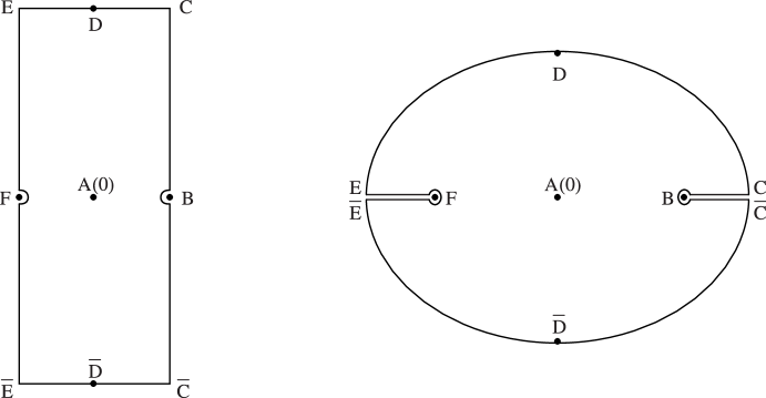
… ►Figure 4.15.7 illustrates the conformal mapping of the strip

-\tfrac{1}{2}\pi<\Re z<\tfrac{1}{2}\pi

onto the whole

w

-plane cut along the real axis from

-\infty

-1

and

1

\infty

, where

w=\sin z

and

z=\operatorname{arcsin}w

(principal value). … ►

See accompanying text — Figure 4.15.7: Conformal mapping of sine and inverse sine. … Magnify

►

§4.15(iii) Complex Arguments: Surfaces

… ►The corresponding surfaces for

\operatorname{arccos}\left(x+iy\right)

\operatorname{arccot}\left(x+iy\right)

\operatorname{arcsec}\left(x+iy\right)

can be visualized from Figures 4.15.9, 4.15.11, 4.15.13 with the aid of equations (4.23.16)–(4.23.18).

26: 3.8 Nonlinear Equations

… ►

Regula Falsi

… ►Inverse linear interpolation (§3.3(v)) is used to obtain the first approximation: … ►

3.8.15

p(x)=(x-1)(x-2)\cdots(x-20)

ⓘ

Permalink:: http://dlmf.nist.gov/3.8.E15
Encodings:: pMML, png, TeX
See also:: Annotations for §3.8(vi), §3.8(vi), §3.8 and Ch.3

… ►Consider

x=20

and

j=19

. We have

p^{\mspace{1.0mu}\prime}(20)=19!

and

a_{19}=1+2+\dots+20=210

. …

27: 8 Incomplete Gamma and Related
Functions

…

28: 28 Mathieu Functions and Hill’s Equation

…

29: 19.10 Relations to Other Functions

… ►

\operatorname{arctan}\left(x/y\right)=xR_{C}\left(y^{2},y^{2}+x^{2}\right),

►

\operatorname{arctanh}\left(x/y\right)=xR_{C}\left(y^{2},y^{2}-x^{2}\right),

►

\operatorname{arcsin}\left(x/y\right)=xR_{C}\left(y^{2}-x^{2},y^{2}\right),

►

\operatorname{arcsinh}\left(x/y\right)=xR_{C}\left(y^{2}+x^{2},y^{2}\right),

… ►For relations to the Gudermannian function

\operatorname{gd}\left(x\right)

and its inverse

{\operatorname{gd}^{-1}}\left(x\right)

(§4.23(viii)), see (19.6.8) and …

30: 8.26 Tables

… ►

•

Khamis (1965) tabulates $P\left(a,x\right)$ for $a=0.05(.05)10(.1)20(.25)70$ , $0.0001\leq x\leq 250$ to 10D.

… ►

•

Abramowitz and Stegun (1964, pp. 245–248) tabulates $E_{n}\left(x\right)$ for $n=2,3,4,10,20$ , $x=0(.01)2$ to 7D; also $(x+n)e^{x}E_{n}\left(x\right)$ for $n=2,3,4,10,20$ , $x^{-1}=0(.01)0.1(.05)0.5$ to 6S.

… ►

•

Pagurova (1961) tabulates $E_{n}\left(x\right)$ for $n=0(1)20$ , $x=0(.01)2(.1)10$ to 4-9S; $e^{x}E_{n}\left(x\right)$ for $n=2(1)10$ , $x=10(.1)20$ to 7D; $e^{x}E_{p}\left(x\right)$ for $p=0(.1)1$ , $x=0.01(.01)7(.05)12(.1)20$ to 7S or 7D.

… ►

•

Zhang and Jin (1996, Table 19.1) tabulates $E_{n}\left(x\right)$ for $n=1,2,3,5,10,15,20$ , $x=0(.1)1,1.5,2,3,5,10,20,30,50,100$ to 7D or 8S.