Mathieu equation
(0.003 seconds)
21—30 of 54 matching pages
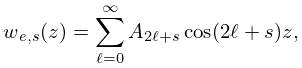
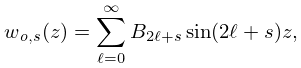
21: 28.14 Fourier Series
…
►
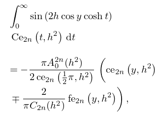
28.14.4
,
…
22: 28.29 Definitions and Basic Properties
…
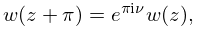
►A generalization of Mathieu’s equation (28.2.1) is Hill’s equation
►
28.29.1
…
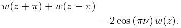
►
28.29.7
…
►
28.29.11
…
►
28.29.13
…
23: 28.32 Mathematical Applications
…
►The separated solutions can be obtained from the modified Mathieu’s equation (28.20.1) for and from Mathieu’s equation (28.2.1) for , where is the separation constant and .
…
►This leads to integral equations and an integral relation between the solutions of Mathieu’s equation (setting , in (28.32.3)).
…
►Let be a solution of Mathieu’s equation (28.2.1) and be a solution of
…defines a solution of Mathieu’s equation, provided that (in the case of an improper curve) the integral converges with respect to uniformly on compact subsets of .
…
►
24: 28.22 Connection Formulas
§28.22 Connection Formulas
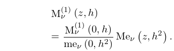
… ►The joining factors in the above formulas are given by … ►
28.22.13
►Here
is given by (28.14.1) with , and is given by (28.24.1) with , , and chosen so that , where the maximum is taken over all integers .
…
►
25: 28.35 Tables
§28.35 Tables
… ►Blanch and Clemm (1969) includes eigenvalues , for , , , ; 4D. Also and for , , and , respectively; 8D. Double points for ; 8D. Graphs are included.
26: Simon Ruijsenaars
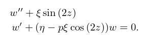
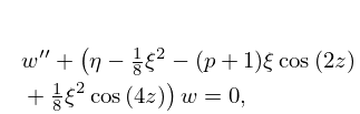
27: 28.31 Equations of Whittaker–Hill and Ince
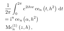
28: 28.28 Integrals, Integral Representations, and Integral Equations
29: Bibliography L
…
►
The solutions of the Mathieu equation with a complex variable and at least one parameter large.
Trans. Amer. Math. Soc. 36 (3), pp. 637–695.
…
►
Algorithm 537: Characteristic values of Mathieu’s differential equation.
ACM Trans. Math. Software 5 (1), pp. 112–117.
…
