Jacobi form

(0.002 seconds)

11—20 of 38 matching pages

11: 29.12 Definitions

… ►With the substitution

\xi={\operatorname{sn}}^{2}\left(z,k\right)

every Lamé polynomial in Table 29.12.1 can be written in the form …

12: 20.14 Methods of Computation

… ►The Fourier series of §20.2(i) usually converge rapidly because of the factors

q^{(n+\frac{1}{2})^{2}}

q^{n^{2}}

, and provide a convenient way of calculating values of

\theta_{j}\left(z\middle|\tau\right)

. Similarly, their

z

-differentiated forms provide a convenient way of calculating the corresponding derivatives. For instance, the first three terms of (20.2.1) give the value of

\theta_{1}\left(2-i\middle|i\right)

(

=\theta_{1}\left(2-i,e^{-\pi}\right)

) to 12 decimal places. … ►For instance, to find

\theta_{3}\left(z,0.9\right)

we use (20.7.32) with

q=0.9=e^{i\pi\tau}

\tau=-i\ln\left(0.9\right)/\pi

. …Hence the first term of the series (20.2.3) for

\theta_{3}\left(z\tau^{\prime}\middle|\tau^{\prime}\right)

suffices for most purposes. …

13: 3.10 Continued Fractions

… ►A continued fraction of the form … ►

Jacobi Fractions

►A continued fraction of the form …is called a Jacobi fraction ( $J$ -fraction). … ►can be written in the form …

14: 29.15 Fourier Series and Chebyshev Series

… ►Since (29.2.5) implies that

\cos\phi=\operatorname{sn}\left(z,k\right)

, (29.15.1) can be rewritten in the form …

15: 20.13 Physical Applications

… ►In the singular limit

\Im\tau\rightarrow 0+

, the functions

\theta_{j}\left(z\middle|\tau\right)

j=1,2,3,4

, become integral kernels of Feynman path integrals (distribution-valued Green’s functions); see Schulman (1981, pp. 194–195). …

16: 29.2 Differential Equations

… ►

§29.2(i) Lamé’s Equation

… ►For

\operatorname{sn}\left(z,k\right)

see §22.2. … ►

§29.2(ii) Other Forms

… ►we have … ►

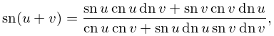
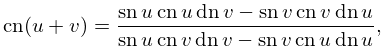
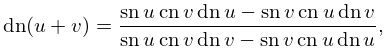
17: 22.8 Addition Theorems

… ►

§22.8(ii) Alternative Forms for Sum of Two Arguments

… ►

22.8.14

\operatorname{sn}(u+v)=\frac{\operatorname{sn}u\operatorname{cn}u\operatorname% {dn}v+\operatorname{sn}v\operatorname{cn}v\operatorname{dn}u}{\operatorname{cn% }u\operatorname{cn}v+\operatorname{sn}u\operatorname{dn}u\operatorname{sn}v% \operatorname{dn}v},

ⓘ

Symbols:: $\operatorname{cn}\left(\NVar{z},\NVar{k}\right)$ : Jacobian elliptic function, $\operatorname{dn}\left(\NVar{z},\NVar{k}\right)$ : Jacobian elliptic function, $\operatorname{sn}\left(\NVar{z},\NVar{k}\right)$ : Jacobian elliptic function, $u$ : complex, $v$ : complex and $k$ : modulus
Permalink:: http://dlmf.nist.gov/22.8.E14
Encodings:: pMML, png, TeX
See also:: Annotations for §22.8(ii), §22.8 and Ch.22

►

22.8.15

\operatorname{cn}(u+v)=\frac{\operatorname{sn}u\operatorname{cn}u\operatorname% {dn}v-\operatorname{sn}v\operatorname{cn}v\operatorname{dn}u}{\operatorname{sn% }u\operatorname{cn}v\operatorname{dn}v-\operatorname{sn}v\operatorname{cn}u% \operatorname{dn}u},

ⓘ

Symbols:: $\operatorname{cn}\left(\NVar{z},\NVar{k}\right)$ : Jacobian elliptic function, $\operatorname{dn}\left(\NVar{z},\NVar{k}\right)$ : Jacobian elliptic function, $\operatorname{sn}\left(\NVar{z},\NVar{k}\right)$ : Jacobian elliptic function, $u$ : complex, $v$ : complex and $k$ : modulus
Permalink:: http://dlmf.nist.gov/22.8.E15
Encodings:: pMML, png, TeX
See also:: Annotations for §22.8(ii), §22.8 and Ch.22

… ►

22.8.17

\operatorname{dn}(u+v)=\frac{\operatorname{sn}u\operatorname{cn}v\operatorname% {dn}u-\operatorname{sn}v\operatorname{cn}u\operatorname{dn}v}{\operatorname{sn% }u\operatorname{cn}v\operatorname{dn}v-\operatorname{sn}v\operatorname{cn}u% \operatorname{dn}u},

ⓘ

Symbols:: $\operatorname{cn}\left(\NVar{z},\NVar{k}\right)$ : Jacobian elliptic function, $\operatorname{dn}\left(\NVar{z},\NVar{k}\right)$ : Jacobian elliptic function, $\operatorname{sn}\left(\NVar{z},\NVar{k}\right)$ : Jacobian elliptic function, $u$ : complex, $v$ : complex and $k$ : modulus
Permalink:: http://dlmf.nist.gov/22.8.E17
Encodings:: pMML, png, TeX
See also:: Annotations for §22.8(ii), §22.8 and Ch.22

… ►

22.8.23

\begin{vmatrix}\operatorname{sn}z_{1}\operatorname{cn}z_{1}&\operatorname{cn}z% _{1}\operatorname{dn}z_{1}&\operatorname{cn}z_{1}&\operatorname{dn}z_{1}\\ \operatorname{sn}z_{2}\operatorname{cn}z_{2}&\operatorname{cn}z_{2}% \operatorname{dn}z_{2}&\operatorname{cn}z_{2}&\operatorname{dn}z_{2}\\ \operatorname{sn}z_{3}\operatorname{cn}z_{3}&\operatorname{cn}z_{3}% \operatorname{dn}z_{3}&\operatorname{cn}z_{3}&\operatorname{dn}z_{3}\\ \operatorname{sn}z_{4}\operatorname{cn}z_{4}&\operatorname{cn}z_{4}% \operatorname{dn}z_{4}&\operatorname{cn}z_{4}&\operatorname{dn}z_{4}\end{% vmatrix}=0.

ⓘ

Symbols:: $\operatorname{cn}\left(\NVar{z},\NVar{k}\right)$ : Jacobian elliptic function, $\operatorname{dn}\left(\NVar{z},\NVar{k}\right)$ : Jacobian elliptic function, $\operatorname{sn}\left(\NVar{z},\NVar{k}\right)$ : Jacobian elliptic function, $\det$ : determinant, $z$ : complex and $k$ : modulus
Permalink:: http://dlmf.nist.gov/22.8.E23
Encodings:: pMML, png, TeX
See also:: Annotations for §22.8(iii), §22.8 and Ch.22

…

18: 18.18 Sums

… ►

Jacobi

… ►

Jacobi

… ►See (18.17.45) and (18.17.49) for integrated forms of (18.18.22) and (18.18.23), respectively. … ►

Jacobi

… ►See also (18.38.3) for a finite sum of Jacobi polynomials. …

19: 18.15 Asymptotic Approximations

… ►

§18.15(i) Jacobi

… ►For large

\beta

, fixed

\alpha

, and

0\leq n/\beta\leq c

, Dunster (1999) gives asymptotic expansions of

P^{(\alpha,\beta)}_{n}\left(z\right)

that are uniform in unbounded complex

z

-domains containing

z=\pm 1

. …This reference also supplies asymptotic expansions of

P^{(\alpha,\beta)}_{n}\left(z\right)

for large

n

, fixed

\alpha

, and

0\leq\beta/n\leq c

. … ►The first term of this expansion also appears in Szegő (1975, Theorem 8.21.7). … ►For asymptotic approximations of Jacobi, ultraspherical, and Laguerre polynomials in terms of Hermite polynomials, see López and Temme (1999a). …

20: 23.15 Definitions

… ►In §§23.15–23.19,

k

and

k^{\prime}

(\in\mathbb{C})

denote the Jacobi modulus and complementary modulus, respectively, and

q=e^{i\pi\tau}

(

\Im\tau>0

) denotes the nome; compare §§20.1 and 22.1. … ►The set of all bilinear transformations of this form is denoted by SL

(2,\mathbb{Z})

(Serre (1973, p. 77)). … ►If, as a function of

q

f(\tau)

is analytic at

q=0

, then

f(\tau)

is called a modular form. If, in addition,

f(\tau)\to 0

q\to 0

, then

f(\tau)

is called a cusp form. …