Heaviside function

SearchAdvancedHelp

(0.002 seconds)

5 matching pages

1: 1.16 Distributions

… ►

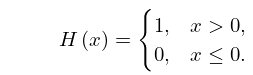
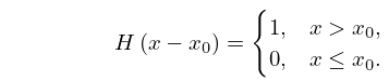
§1.16(iv) Heaviside Function

►

1.16.13

ⓘ

Defines:

$H\left(x\right)$: Heaviside function

Referenced by:

§1.14(iii), §1.16(viii), §18.40(ii)

Permalink:

http://dlmf.nist.gov/1.16.E13

Encodings:

pMML, png, TeX

See also:

Annotations for §1.16(iv), §1.16 and Ch.1

►

1.16.14

ⓘ

Symbols:

$H\left(x\right)$: Heaviside function

Referenced by:

§1.4(v)

Permalink:

http://dlmf.nist.gov/1.16.E14

Encodings:

pMML, png, TeX

See also:

Annotations for §1.16(iv), §1.16 and Ch.1

… ►

1.16.44 $$\mathrm{sign}\left(x\right)=2H\left(x\right)-1,$$ $x\ne 0$,

ⓘ

Symbols:

$H\left(x\right)$: Heaviside function and $\mathrm{sign}x$: sign of

Permalink:

http://dlmf.nist.gov/1.16.E44

Encodings:

pMML, png, TeX

See also:

Annotations for §1.16(viii), §1.16 and Ch.1

… ►where $H\left(x\right)$ is the Heaviside function defined in (1.16.13), and the derivatives are to be understood in the sense of distributions. …

2: 18.40 Methods of Computation

… ►

18.40.7 $${\mu }_N(x)=\sum _{n=1}^N{w}_{n}H\left(x-x_n\right),$$ $x\in (a,b)$,

ⓘ

Symbols:

$H\left(x\right)$: Heaviside function, $\in$: element of, $(a,b)$: open interval, $N$: positive integer, $w_x$: weights, $n$: nonnegative integer and $x$: real variable

Source:

Shohat and Tamarkin (1970, pp. 42-43)

Referenced by:

§18.40(ii)

Permalink:

http://dlmf.nist.gov/18.40.E7

Encodings:

pMML, png, TeX

See also:

Annotations for §18.40(ii), §18.40(ii), §18.40 and Ch.18

► $H\left(x\right)$ being the Heaviside step-function, see (1.16.13). …

3: 2.6 Distributional Methods

… ►

2.6.37 $$F\ast G={𝐷}^{n+m}(f\ast g).$$

ⓘ

Symbols:

$g(t)$: locally integrable function, $\ast$: convolution, $𝐷$: derivative of distribution, $f(t)$: locally integrable function, $n$: nonnegative integer, $F$: derivative and $G$: derivative

Referenced by:

§2.6(iii)

Permalink:

http://dlmf.nist.gov/2.6.E37

Encodings:

pMML, png, TeX

See also:

Annotations for §2.6(iii), §2.6 and Ch.2

… ►Furthermore, $K^{+}$ contains the distributions $H$, $\delta$, and $t^{\lambda }$, $t>0$, for any real (or complex) number $\lambda$, where $H$ is the distribution associated with the Heaviside function $H\left(t\right)$ (§1.16(iv)), and $t^{\lambda }$ is the distribution defined by (2.6.12)–(2.6.14), depending on the value of $\lambda$. …

4: 1.14 Integral Transforms

… ►

1.14.22 $$ℒf_a^{+}\left(s\right)={\mathrm{e}}^{-as}ℒf\left(s\right),$$

ⓘ

Symbols:

$H\left(x\right)$: Heaviside function, $ℒ\left(f\right)\left(s\right)$: Laplace transform and $\mathrm{e}$: base of natural logarithm

Keywords:

Laplace transform

Permalink:

http://dlmf.nist.gov/1.14.E22

Encodings:

pMML, png, TeX

Notational Change (effective with 1.0.15):

The notation for the Laplace transform was changed to $ℒ\left(f\right)\left(s\right)$ from $ℒ(f(t);s)$. In addition, the auxiliary function $f_a^{+}(t)=H\left(t-a\right)f(t-a)$ was introduced.

See also:

Annotations for §1.14(iii), §1.14(iii), §1.14 and Ch.1

►where $f_a^{+}(t)=H\left(t-a\right)f(t-a)$ and $H$ is the Heaviside function; see (1.16.13). …

5: 1.4 Calculus of One Variable

… ►If, for example, $\alpha (x)=H\left(x-x_n\right)$, the Heaviside unit step-function (1.16.14), then the corresponding measure $d\alpha (x)$ is $\delta \left(x-x_n\right)dx$, where $\delta \left(x-x_n\right)$ is the Dirac $\delta$-function of §1.17, such that, for $f(x)$ a continuous function on $(a,b)$, ${\int }_a^{b}f(x)d\alpha (x)=f(x_n)$ for $x_n\in (a,b)$ and $0$ otherwise. …