Fiat%20Wallet%20Customer%201-201-63O-7680%20Support%20Number%20Fiat%20Wallet%20Helpline%20Toll%20
(0.006 seconds)
21—30 of 291 matching pages
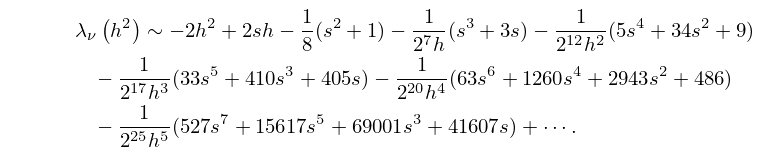
21: 28.16 Asymptotic Expansions for Large
22: 27.2 Functions
§27.2(ii) Tables
…23: 7.24 Approximations
Cody (1969) provides minimax rational approximations for and . The maximum relative precision is about 20S.
Cody et al. (1970) gives minimax rational approximations to Dawson’s integral (maximum relative precision 20S–22S).
24: 25.3 Graphics
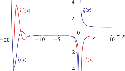
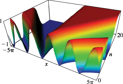
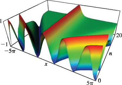
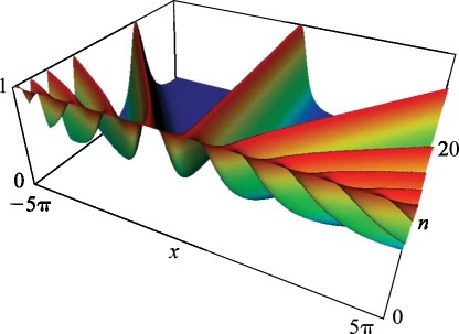
25: 25.12 Polylogarithms
 ►
►

26: 9.18 Tables
Miller (1946) tabulates , for , for ; , for ; , for ; , , , (respectively , , , ) for . Precision is generally 8D; slightly less for some of the auxiliary functions. Extracts from these tables are included in Abramowitz and Stegun (1964, Chapter 10), together with some auxiliary functions for large arguments.
Zhang and Jin (1996, p. 337) tabulates , , , for to 8S and for to 9D.
Sherry (1959) tabulates , , , , ; 20S.
Zhang and Jin (1996, p. 339) tabulates , , , , , , , , ; 8D.
27: Tom M. Apostol
28: 25.20 Approximations
Cody et al. (1971) gives rational approximations for in the form of quotients of polynomials or quotients of Chebyshev series. The ranges covered are , , , . Precision is varied, with a maximum of 20S.
29: 28.35 Tables
Ince (1932) includes eigenvalues , , and Fourier coefficients for or , ; 7D. Also , for , , corresponding to the eigenvalues in the tables; 5D. Notation: , .
Kirkpatrick (1960) contains tables of the modified functions , for , , ; 4D or 5D.
National Bureau of Standards (1967) includes the eigenvalues , for with , and with ; Fourier coefficients for and for , , respectively, and various values of in the interval ; joining factors , for with (but in a different notation). Also, eigenvalues for large values of . Precision is generally 8D.
Zhang and Jin (1996, pp. 521–532) includes the eigenvalues , for , ; (’s) or 19 (’s), . Fourier coefficients for , , . Mathieu functions , , and their first -derivatives for , . Modified Mathieu functions , , and their first -derivatives for , , . Precision is mostly 9S.
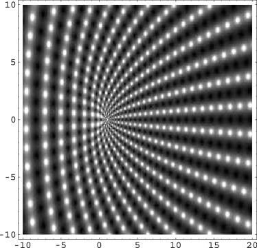
30: 22.3 Graphics
 ►
►
