Dirichlet%20product%20%28or%20convolution%29

SearchAdvancedHelp

(0.002 seconds)

11—20 of 297 matching pages

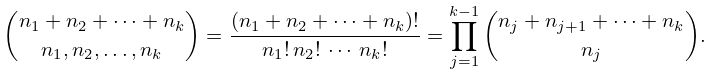
11: 26.4 Lattice Paths: Multinomial Coefficients and Set Partitions

… ►

26.4.2 $$\left(\genfrac{}{}{0.0pt}{}{n_1+n_2+\mathrm{\cdots }+n_k}{n_1,n_2,\mathrm{\dots },n_k}\right)=\frac{(n_1+n_2+\mathrm{\cdots }+n_k)!}{n_1!n_2!\mathrm{\cdots }{n}_k!}=\prod _{j=1}^{k-1}\left(\genfrac{}{}{0.0pt}{}{n_j+n_{j+1}+\mathrm{\cdots }+n_k}{n_j}\right).$$

ⓘ

Symbols:

$\left(\genfrac{}{}{0.0pt}{}{m}{n}\right)$: binomial coefficient, $!$: factorial (as in $n!$), $\left(\genfrac{}{}{0.0pt}{}{n_1+n_2+\mathrm{\cdots }+n_k}{n_1,n_2,\mathrm{\dots },n_k}\right)$: multinomial coefficient, $j$: nonnegative integer, $k$: nonnegative integer and $n$: nonnegative integer

A&S Ref:

24.1.2

Referenced by:

§26.4(i)

Permalink:

http://dlmf.nist.gov/26.4.E2

Encodings:

pMML, png, TeX

See also:

Annotations for §26.4(i), §26.4 and Ch.26

… ►

Table 26.4.1: Multinomials and partitions.

► ►►►►

$n$	$m$	$\lambda$	$M_1$	$M_2$	$M_3$
…
$5$	$2$	$2^1,3^1$	$10$	$20$	$10$
$5$	$3$	$1^2,3^1$	$20$	$20$	$10$
…

►

…

12: 27.15 Chinese Remainder Theorem

… ►The Chinese remainder theorem states that a system of congruences $x\equiv a_1(mod{m}_1),\mathrm{\dots },x\equiv a_k(mod{m}_k)$, always has a solution if the moduli are relatively prime in pairs; the solution is unique (mod $m$), where $m$ is the product of the moduli. … ►Their product $m$ has 20 digits, twice the number of digits in the data. …These numbers, in turn, are combined by the Chinese remainder theorem to obtain the final result $(modm)$, which is correct to 20 digits. …

13: 8 Incomplete Gamma and Related
Functions

…

14: Bibliography M

… ►

Rational approximations, software and test methods for sine and cosine integrals. Numer. Algorithms 12 (3-4), pp. 259–272.

ⓘ

Notes:

Includes Fortran code, maximum accuracy 20S.

External Links:

ISSN 1017-1398, Document, MathReview, ZentralBlatt

Referenced by:

§6.13, 4th item, §6.21(ii).

Encodings:

BibTeX

… ►

Hill’s Equation. Interscience Tracts in Pure and Applied Mathematics, No. 20, Interscience Publishers John Wiley & Sons, New York-London-Sydney.

ⓘ

Notes:

Reprinted by Dover Publications, Inc., New York, 1979.

External Links:

MathReview (H. Hochstadt), ZentralBlatt

Referenced by:

§1.3(iii), §28.29(i), §28.29(ii), §28.29(ii), §28.29(iii), §28.29(iii), §28.29(iii), §28.30(i), Ch.28, §29.3(i), §29.9.

Encodings:

BibTeX

… ►

Calculation of the modified Bessel functions of the second kind with complex argument. Math. Comp. 20 (95), pp. 407–412.

ⓘ

External Links:

ISSN 0025-5718, FullText, MathReview (H. E. Fettis), ZentralBlatt

Referenced by:

§10.74(iii).

Encodings:

BibTeX

… ►

Hierarchies and logarithmic oscillations in the temporal relaxation patterns of proteins and other complex systems. Proc. Nat. Acad. Sci. U .S. A. 96 (20), pp. 11085–11089.

ⓘ

External Links:

FullText

Referenced by:

§8.24(i).

Encodings:

BibTeX

… ►

The $q$-analogue of the Laguerre polynomials. J. Math. Anal. Appl. 81 (1), pp. 20–47.

ⓘ

External Links:

ISSN 0022-247X, Document, MathReview (R. A. Askey), ZentralBlatt

Referenced by:

§18.27(v).

Encodings:

BibTeX

…

15: 8.26 Tables

… ►

Khamis (1965) tabulates $P(a,x)$ for $a=0.05(.05)10(.1)20(.25)70$, $0.0001\le x\le 250$ to 10D.

… ►

Abramowitz and Stegun (1964, pp. 245–248) tabulates $E_n\left(x\right)$ for $n=2,3,4,10,20$, $x=0(.01)2$ to 7D; also $(x+n){\mathrm{e}}^x{E}_n\left(x\right)$ for $n=2,3,4,10,20$, $x^{-1}=0(.01)0.1(.05)0.5$ to 6S.

… ►

Pagurova (1961) tabulates $E_n\left(x\right)$ for $n=0(1)20$, $x=0(.01)2(.1)10$ to 4-9S; ${\mathrm{e}}^x{E}_n\left(x\right)$ for $n=2(1)10$, $x=10(.1)20$ to 7D; ${\mathrm{e}}^x{E}_p\left(x\right)$ for $p=0(.1)1$, $x=0.01(.01)7(.05)12(.1)20$ to 7S or 7D.

… ►

Zhang and Jin (1996, Table 19.1) tabulates $E_n\left(x\right)$ for $n=1,2,3,5,10,15,20$, $x=0(.1)1,1.5,2,3,5,10,20,30,50,100$ to 7D or 8S.

16: 23 Weierstrass Elliptic and Modular
Functions

…

17: 10.75 Tables

… ►

Achenbach (1986) tabulates $J_0\left(x\right)$, $J_1\left(x\right)$, $Y_0\left(x\right)$, $Y_1\left(x\right)$, $x=0(.1)8$, 20D or 18–20S.

… ►

Makinouchi (1966) tabulates all values of $j_{\nu ,m}$ and $y_{\nu ,m}$ in the interval $(0,100)$, with at least 29S. These are for $\nu =0(1)5$, 10, 20; $\nu =\frac{3}{2}$, $\frac{5}{2}$; $\nu =m/n$ with $m=1(1)n-1$ and $n=3(1)8$, except for $\nu =\frac{1}{2}$.

… ►

Bickley et al. (1952) tabulates $x^{-n}{I}_n\left(x\right)$ or ${\mathrm{e}}^{-x}{I}_n\left(x\right)$, $x^n{K}_n\left(x\right)$ or ${\mathrm{e}}^x{K}_n\left(x\right)$, $n=2(1)20$, $x=0$(.01 or .1) 10(.1) 20, 8S; $I_n\left(x\right)$, $K_n\left(x\right)$, $n=0(1)20$, $x=0$ or $0.1(.1)20$, 10S.

… ►

Kerimov and Skorokhodov (1984b) tabulates all zeros of the principal values of $K_n\left(z\right)$ and $K_n^{\prime }\left(z\right)$, for $n=2(1)20$, 9S.

… ►

Zhang and Jin (1996, p. 322) tabulates $\mathrm{ber}x$, ${\mathrm{ber}}^{\prime }x$, $\mathrm{bei}x$, ${\mathrm{bei}}^{\prime }x$, $\ker x$, ${\ker }^{\prime }x$, $\mathrm{kei}x$, ${\mathrm{kei}}^{\prime }x$, $x=0(1)20$, 7S.

…

18: Publications

… ►

Web-Based 3D Visualization in a Digital Library of Mathematical Functions, Proceedings of the Web3D Symposium, Bangor, UK, March 29–April 1, 2005.

►

From B-Spline Mesh Generation to Effective Visualizations for the NIST Digital Library of Mathematical Functions, in Curve and Surface Design, Proceedings of the Sixth International Conference on Curves and Surfaces, Avignon, France June 29–July 5, 2006, pp. 235–243.

… ►

Tensor Product B-Spline Mesh Generation for Accurate Surface Visualizations in the NIST Digital Library of Mathematical Functions, in Mathematical Methods for Curves and Surfaces, Proceedings of the 2008 International Conference on Mathematical Methods for Curves and Surfaces (MMCS 2008), Lecture Notes in Computer Science, Vol. 5862, (M. Dæhlen, M. Floater., T. Lyche, J. L. Merrien, K. Mørken, L. L. Schumaker, eds), Springer, Berlin, Heidelberg (2010) pp. 385–393.

… ►

NIST’s Digital Library of Mathematial Functions, Physics Today 71, 2, 48 (2018), pp. 48–53.

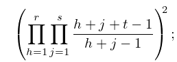
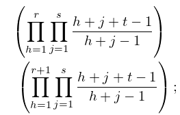
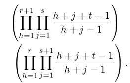
19: 26.12 Plane Partitions

… ►

Table 26.12.1: Plane partitions.

► ►►►

$n$	$\mathrm{pp}\left(n\right)$	$n$	$\mathrm{pp}\left(n\right)$	$n$	$\mathrm{pp}\left(n\right)$
…
3	6	20	75278	37	903 79784
…

►

… ►

26.12.9 $${\left(\prod _{h=1}^r\prod _{j=1}^s\frac{h+j+t-1}{h+j-1}\right)}^2;$$

ⓘ

Symbols:

$r$: positive integer, $s$: positive integer, $t$: positive integer, $h$: positive integer and $j$: positive integer

Permalink:

http://dlmf.nist.gov/26.12.E9

Encodings:

pMML, png, TeX

See also:

Annotations for §26.12(i), §26.12 and Ch.26

… ►

26.12.10 $$\left(\prod _{h=1}^r\prod _{j=1}^s\frac{h+j+t-1}{h+j-1}\right)\left(\prod _{h=1}^{r+1}\prod _{j=1}^s\frac{h+j+t-1}{h+j-1}\right);$$

ⓘ

Symbols:

$r$: positive integer, $s$: positive integer, $t$: positive integer, $h$: positive integer and $j$: positive integer

Permalink:

http://dlmf.nist.gov/26.12.E10

Encodings:

pMML, png, TeX

See also:

Annotations for §26.12(i), §26.12 and Ch.26

… ►

26.12.11 $$\left(\prod _{h=1}^{r+1}\prod _{j=1}^s\frac{h+j+t-1}{h+j-1}\right)\left(\prod _{h=1}^r\prod _{j=1}^{s+1}\frac{h+j+t-1}{h+j-1}\right).$$

ⓘ

Symbols:

$r$: positive integer, $s$: positive integer, $t$: positive integer, $h$: positive integer and $j$: positive integer

Permalink:

http://dlmf.nist.gov/26.12.E11

Encodings:

pMML, png, TeX

See also:

Annotations for §26.12(i), §26.12 and Ch.26

… ►

26.12.13 $$\prod _{h=1}^r\prod _{j=1}^r\frac{h+j+t-1}{h+j-1};$$

ⓘ

Symbols:

$r$: positive integer, $t$: positive integer, $h$: positive integer and $j$: positive integer

Permalink:

http://dlmf.nist.gov/26.12.E13

Encodings:

pMML, png, TeX

See also:

Annotations for §26.12(i), §26.12 and Ch.26

…

20: 36 Integrals with Coalescing Saddles

…