…
►Also let
and
(§
18.3).
…
►
…
►
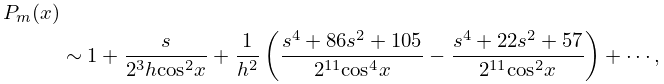
28.8.11
…
►The approximations are expressed in terms of Whittaker functions
and
with
; compare §
2.8(vi).
…
►Subsequently the asymptotic solutions involving either elementary or Whittaker functions are identified in terms of the Floquet solutions
(§
28.12(ii)) and modified Mathieu functions
(§
28.20(iii)).
…
…
►with
and all allowable choices of
,
,
, and
.
…
►Let
with
and
.
…The integers
,
, and
are characteristics of the machine.
…
►
, and
…Then
rounding by chopping or
rounding down of
gives
, with maximum relative error
.
…
…
►For the generalized hypergeometric function
see (
16.2.1).
…
►Define operators
and
acting on symmetric Laurent polynomials by
(
given by (
18.28.6_2)) and
.
…commutes with
, that is
, and satisfies
…where
is a constant with explicit expression in terms of
and
given in
Koornwinder (2007a, (2.8)).
►The abstract associative algebra with generators
and relations (
18.38.4), (
18.38.6) and with the constants
in (
18.38.6) not yet specified, is called the
Zhedanov algebra or
Askey–Wilson algebra AW(3).
…
…
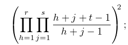
►
26.12.9
…
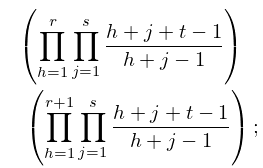
►
26.12.10
…
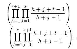
►
26.12.11
…
►The notation
denotes the sum over all plane partitions contained in
, and
denotes the number of elements in
.
…
►where
is the sum of the squares of the divisors of
.
…
…
►
denotes the set of permutations of
.
is a one-to-one and onto mapping from
to itself.
…
►An element of
with
fixed points,
cycles of length
cycles of length
, where
, is said to have
cycle type
.
The number of elements of
with cycle type
is given by (
26.4.7).
…
►A permutation with cycle type
can be written as a product of
transpositions, and no fewer.
…

