.2019%E4%BD%93%E6%93%8D%E4%B8%96%E7%95%8C%E6%9D%AF%E3%80%8Ewn4.com%E3%80%8F%E4%BC%AA%E7%90%83%E8%BF%B7%E4%B8%96%E7%95%8C%E6%9D%AF%E6%AE%B5%E5%AD%90.w6n2c9o.2022%E5%B9%B411%E6%9C%8830%E6%97%A511%E6%97%B644%E5%88%8622%E7%A7%92.8ekw666qq

(0.020 seconds)

11—20 of 597 matching pages

11: Bibliography S

… ►

F. W. Schäfke and D. Schmidt (1966) Ein Verfahren zur Berechnung des charakteristischen Exponenten der Mathieuschen Differentialgleichung III. Numer. Math. 8 (1), pp. 68–71.

ⓘ

Notes:: Includes Algol program
External Links:: ISSN 0029-599X, Document, MathReview (S. C. van Veen), ZentralBlatt
Referenced by:: §28.36(ii).
Encodings:: BibTeX

… ►

J. B. Seaborn (1991) Hypergeometric Functions and Their Applications. Texts in Applied Mathematics, Vol. 8, Springer-Verlag, New York.

ⓘ

External Links:: ISBN 0-387-97558-6, MathReview (Wolfgang Bühring), ZentralBlatt
Referenced by:: Erratum (V1.2.0) Section 18.39.
Encodings:: BibTeX

… ►

R. Shail (1978) Lamé polynomial solutions to some elliptic crack and punch problems. Internat. J. Engrg. Sci. 16 (8), pp. 551–563.

ⓘ

External Links:: ISSN 0020-7225, Document, MathReview, ZentralBlatt
Referenced by:: §29.19(ii).
Encodings:: BibTeX

… ►

R. Sips (1949) Représentation asymptotique des fonctions de Mathieu et des fonctions d’onde sphéroidales. Trans. Amer. Math. Soc. 66 (1), pp. 93–134 (French).

ⓘ

External Links:: FullText, MathReview (M. Strutt), ZentralBlatt
Referenced by:: §28.8(ii).
Encodings:: BibTeX

… ►

R. Sips (1967) Répartition du courant alternatif dans un conducteur cylindrique de section elliptique. Acad. Roy. Belg. Bull. Cl. Sci. (5) 53 (8), pp. 861–878.

ⓘ

Referenced by:: 6th item.
Encodings:: BibTeX

…

12: Bibliography K

… ►

E. H. Kaufman and T. D. Lenker (1986) Linear convergence and the bisection algorithm. Amer. Math. Monthly 93 (1), pp. 48–51.

ⓘ

External Links:: ISSN 0002-9890, FullText, MathReview (J. G. Herriot), ZentralBlatt
Referenced by:: §3.8(iii).
Encodings:: BibTeX

… ►

N. D. Kazarinoff (1988) Special functions and the Bieberbach conjecture. Amer. Math. Monthly 95 (8), pp. 689–696.

ⓘ

External Links:: ISSN 0002-9890, FullText, MathReview (S. L. Shukla), ZentralBlatt
Referenced by:: §16.23(iii).
Encodings:: BibTeX

… ►

M. K. Kerimov and S. L. Skorokhodov (1984b) Calculation of the complex zeros of the modified Bessel function of the second kind and its derivatives. Zh. Vychisl. Mat. i Mat. Fiz. 24 (8), pp. 1150–1163.

ⓘ

Notes:: English translation in U.S.S.R. Computational Math. and Math. Phys. 24(4), pp. 115–123
External Links:: ISSN 0044-4669, Document, MathReview (Walter Gautschi), ZentralBlatt
Referenced by:: §10.42, §10.74(vi), 3rd item.
Encodings:: BibTeX

… ►

T. H. Koornwinder (1977) The addition formula for Laguerre polynomials. SIAM J. Math. Anal. 8 (3), pp. 535–540.

ⓘ

External Links:: Document, MathReview (M. Mikolas), ZentralBlatt
Referenced by:: (18.14.8), §18.14(i), §18.17(ii), §18.18(ii).
Encodings:: BibTeX

… ►

B. G. Korenev (2002) Bessel Functions and their Applications. Analytical Methods and Special Functions, Vol. 8, Taylor & Francis Ltd., London-New York.

ⓘ

Notes:: Translated from the Russian by E. V. Pankratiev
External Links:: ISBN 0-415-28130-X, MathReview (L. Debnath), ZentralBlatt
Referenced by:: §10.73(i), §10.73(i), §10.73(i).
Encodings:: BibTeX

…

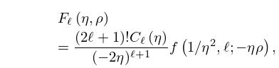
13: 33.16 Connection Formulas

… ►

§33.16(i) $F_{\ell}$ and $G_{\ell}$ in Terms of $f$ and $h$

►

33.16.1

F_{\ell}\left(\eta,\rho\right)=\dfrac{(2\ell+1)!C_{\ell}\left(\eta\right)}{(-2% \eta)^{\ell+1}}f\left(1/\eta^{2},\ell;-\eta\rho\right),

ⓘ

Symbols:: $C_{\NVar{\ell}}\left(\NVar{\eta}\right)$ : normalizing constant for Coulomb radial functions, $f\left(\NVar{\epsilon},\NVar{\ell};\NVar{r}\right)$ : regular Coulomb function, $!$ : factorial (as in $n!$ ), $F_{\NVar{\ell}}\left(\NVar{\eta},\NVar{\rho}\right)$ : regular Coulomb radial function, $\ell$ : nonnegative integer, $\rho$ : nonnegative real variable and $\eta$ : real parameter
Referenced by:: §33.18
Permalink:: http://dlmf.nist.gov/33.16.E1
Encodings:: pMML, png, TeX
See also:: Annotations for §33.16(i), §33.16 and Ch.33

… ►where

C_{\ell}\left(\eta\right)

is given by (33.2.5) or (33.2.6). ►

§33.16(ii) $f$ and $h$ in Terms of $F_{\ell}$ and $G_{\ell}$ when $\epsilon>0$

… ►

§33.16(iv) $s$ and $c$ in Terms of $F_{\ell}$ and $G_{\ell}$ when $\epsilon>0$

…

14: 1.14 Integral Transforms

… ►In this subsection we let

F(x)=\mathscr{F}\left(f\right)\left(x\right)

. ►If

f(t)

is absolutely integrable on

(-\infty,\infty)

, then

F(x)

is continuous,

F(x)\to 0

x\to\pm\infty

, and … ►If

f(t)

and

g(t)

are absolutely integrable on

(-\infty,\infty)

, then so is

(f*g)(t)

, and its Fourier transform is

F(x)G(x)

, where

G(x)

is the Fourier transform of

g(t)

. … ►If

f(t)

and

g(t)

are continuous and absolutely integrable on

(-\infty,\infty)

, and

F(x)=G(x)

for all

x

, then

f(t)=g(t)

for all

t

. … ►In this subsection we let

F_{c}(x)=\mathscr{F}_{\mkern-3.0muc}\mskip-1.0muf\mskip 3.0mu\left(x\right)

F_{s}(x)=\mathscr{F}_{\mkern-2.0mus}\mskip-1.0muf\mskip 3.0mu\left(x\right)

G_{c}(x)=\mathscr{F}_{\mkern-3.0muc}\mskip-1.0mug\mskip 3.0mu\left(x\right)

, and

G_{s}(x)=\mathscr{F}_{\mkern-2.0mus}\mskip-1.0mug\mskip 3.0mu\left(x\right)

. …

15: 8 Incomplete Gamma and Related
Functions

Chapter 8 Incomplete Gamma and Related Functions

…

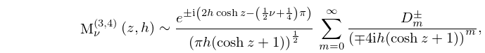
16: 28.25 Asymptotic Expansions for Large $\Re z$

… ►

28.25.1

{\operatorname{M}^{(3,4)}_{\nu}}\left(z,h\right)\sim\frac{e^{\pm\mathrm{i}% \left(2h\cosh z-\left(\frac{1}{2}\nu+\frac{1}{4}\right)\pi\right)}}{\left(\pi h% (\cosh z+1)\right)^{\frac{1}{2}}}\*\sum_{m=0}^{\infty}\dfrac{D^{\pm}_{m}}{% \left(\mp 4\mathrm{i}h(\cosh z+1)\right)^{m}},

ⓘ

Symbols:: $\sim$ : Poincaré asymptotic expansion, $\pi$ : the ratio of the circumference of a circle to its diameter, $\mathrm{e}$ : base of natural logarithm, $\cosh\NVar{z}$ : hyperbolic cosine function, $\mathrm{i}$ : imaginary unit, ${\operatorname{M}^{(\NVar{j})}_{\NVar{\nu}}}\left(\NVar{z},\NVar{h}\right)$ : modified Mathieu function, $m$ : integer, $h$ : parameter, $z$ : complex variable, $\nu$ : complex parameter and $D_{m}^{\pm}$ : coefficients
A&S Ref:: 20.9.1 (for 3 and for integer $\nu$ ) 20.9.3 (for 4 and for integer $\nu$ )
Referenced by:: §28.25
Permalink:: http://dlmf.nist.gov/28.25.E1
Encodings:: pMML, png, TeX
See also:: Annotations for §28.25 and Ch.28

… ►

D_{-1}^{\pm}=0,

►

D_{0}^{\pm}=1,

… ►

28.25.3

(m+1)D^{\pm}_{m+1}+{\left((m+\tfrac{1}{2})^{2}\pm(m+\tfrac{1}{4})8\mathrm{i}h+% 2h^{2}-a\right)D^{\pm}_{m}}\pm(m-\tfrac{1}{2})\left(8\mathrm{i}hm\right)D_{m-1% }^{\pm}=0,

m\geq 0

ⓘ

Symbols:: $\mathrm{i}$ : imaginary unit, $m$ : integer, $h$ : parameter, $a$ : parameter and $D_{m}^{\pm}$ : coefficients
A&S Ref:: 20.9.2 (for $+$ ) 20.9.4 (for $-$ )
Permalink:: http://dlmf.nist.gov/28.25.E3
Encodings:: pMML, png, TeX
See also:: Annotations for §28.25 and Ch.28

…

17: 26.10 Integer Partitions: Other Restrictions

… ►

p\left(\mathcal{D},n\right)

denotes the number of partitions of

n

into distinct parts.

p_{m}\left(\mathcal{D},n\right)

denotes the number of partitions of

n

into at most

m

distinct parts.

p\left(\mathcal{D}k,n\right)

denotes the number of partitions of

n

into parts with difference at least

k

. …If more than one restriction applies, then the restrictions are separated by commas, for example,

p\left(\mathcal{D}2,\hbox{}\!\!\in\!T,n\right)

. … ►Note that

p\left(\mathcal{D}^{\prime}3,n\right)\leq p\left(\mathcal{D}3,n\right)

, with strict inequality for

n\geq 9

. …

18: 26.6 Other Lattice Path Numbers

… ►

Delannoy Number $D(m,n)$

►

D(m,n)

is the number of paths from

(0,0)

(m,n)

that are composed of directed line segments of the form

(1,0)

(0,1)

, or

(1,1)

. … ►

Table 26.6.1: Delannoy numbers

D(m,n)

► ►►

$m$	$n$
$m$	…

► … ►

26.6.4

r(n)=D(n,n)-D(n+1,n-1),

n\geq 1

ⓘ

Defines:: $r(n)$ : Schröder number (locally)
Symbols:: $n$ : nonnegative integer and $D(m,n)$ : Delannoy number
Referenced by:: §26.6(i)
Permalink:: http://dlmf.nist.gov/26.6.E4
Encodings:: pMML, png, TeX
See also:: Annotations for §26.6(i), §26.6(i), §26.6 and Ch.26

… ►

26.6.10

D(m,n)=D(m,n-1)+D(m-1,n)+D(m-1,n-1),

m,n\geq 1

ⓘ

Symbols:: $m$ : nonnegative integer, $n$ : nonnegative integer and $D(m,n)$ : Delannoy number
Referenced by:: §26.6(iii)
Permalink:: http://dlmf.nist.gov/26.6.E10
Encodings:: pMML, png, TeX
See also:: Annotations for §26.6(iii), §26.6 and Ch.26

…

19: 1.11 Zeros of Polynomials

… ►Set

z=w-\tfrac{1}{3}a

to reduce

f(z)=z^{3}+az^{2}+bz+c

g(w)=w^{3}+pw+q

, with

p=(3b-a^{2})/3

q=(2a^{3}-9ab+27c)/27

. … ►

p=(-3a^{2}+8b)/8,

… ►Resolvent cubic is

z^{3}+12z^{2}+20z+9=0

with roots

\theta_{1}=-1

\theta_{2}=-\tfrac{1}{2}(11+\sqrt{85})

\theta_{3}=-\tfrac{1}{2}(11-\sqrt{85})

, and

\sqrt{-\theta_{1}}=1

\sqrt{-\theta_{2}}=\tfrac{1}{2}(\sqrt{17}+\sqrt{5})

\sqrt{-\theta_{3}}=\tfrac{1}{2}(\sqrt{17}-\sqrt{5})

. … ►Let … ►Then

f(z)

, with

a_{n}\not=0

, is stable iff

a_{0}\not=0

;

D_{2k}>0

k=1,\dots,\left\lfloor\frac{1}{2}n\right\rfloor

;

\operatorname{sign}D_{2k+1}=\operatorname{sign}a_{0}

k=0,1,\dots,\left\lfloor\frac{1}{2}n-\frac{1}{2}\right\rfloor

20: 21.5 Modular Transformations

… ►Let

\mathbf{A}

\mathbf{B}

\mathbf{C}

, and

\mathbf{D}

g\times g

matrices with integer elements such that ►

21.5.1

\boldsymbol{{\Gamma}}=\begin{bmatrix}\mathbf{A}&\mathbf{B}\\ \mathbf{C}&\mathbf{D}\end{bmatrix}

ⓘ

Defines:: Matrix $\boldsymbol{{\Gamma}}$ (locally)
Permalink:: http://dlmf.nist.gov/21.5.E1
Encodings:: pMML, png, TeX
See also:: Annotations for §21.5(i), §21.5 and Ch.21

… ►

21.5.4

\theta\left(\left[[\mathbf{C}\boldsymbol{{\Omega}}+\mathbf{D}]^{-1}\right]^{% \mathrm{T}}\mathbf{z}\middle|[\mathbf{A}\boldsymbol{{\Omega}}+\mathbf{B}][% \mathbf{C}\boldsymbol{{\Omega}}+\mathbf{D}]^{-1}\right)=\xi(\boldsymbol{{% \Gamma}})\sqrt{\det[\mathbf{C}\boldsymbol{{\Omega}}+\mathbf{D}]}e^{\pi i% \mathbf{z}\cdot\left[[\mathbf{C}\boldsymbol{{\Omega}}+\mathbf{D}]^{-1}\mathbf{% C}\right]\cdot\mathbf{z}}\theta\left(\mathbf{z}\middle|\boldsymbol{{\Omega}}% \right).

ⓘ

Symbols:: $\theta\left(\NVar{\mathbf{z}}\middle|\NVar{\boldsymbol{{\Omega}}}\right)$ : Riemann theta function, $\pi$ : the ratio of the circumference of a circle to its diameter, $\det$ : determinant, $\mathrm{e}$ : base of natural logarithm, $\mathrm{i}$ : imaginary unit, $\NVar{\mathbf{A}}^{\mathrm{T}}$ : transpose of matrix, $\boldsymbol{{\Omega}}$ : a Riemann matrix, Matrix $\boldsymbol{{\Gamma}}$ and $\xi(\boldsymbol{{\Gamma}})$ : eighth root of unity
Referenced by:: §21.5(i)
Permalink:: http://dlmf.nist.gov/21.5.E4
Encodings:: pMML, png, TeX
See also:: Annotations for §21.5(i), §21.5 and Ch.21

►Here

\xi(\boldsymbol{{\Gamma}})

is an eighth root of unity, that is,

(\xi(\boldsymbol{{\Gamma}}))^{8}=1

. … ►

21.5.9

\theta\genfrac{[}{]}{0.0pt}{}{\mathbf{D}\boldsymbol{{\alpha}}-\mathbf{C}% \boldsymbol{{\beta}}+\tfrac{1}{2}\operatorname{diag}[\mathbf{C}\mathbf{D}^{% \mathrm{T}}]}{-\mathbf{B}\boldsymbol{{\alpha}}+\mathbf{A}\boldsymbol{{\beta}}+% \tfrac{1}{2}\operatorname{diag}[\mathbf{A}\mathbf{B}^{\mathrm{T}}]}\left(\left% [[\mathbf{C}\boldsymbol{{\Omega}}+\mathbf{D}]^{-1}\right]^{\mathrm{T}}\mathbf{% z}\middle|[\mathbf{A}\boldsymbol{{\Omega}}+\mathbf{B}][\mathbf{C}\boldsymbol{{% \Omega}}+\mathbf{D}]^{-1}\right)=\kappa(\boldsymbol{{\alpha}},\boldsymbol{{% \beta}},\boldsymbol{{\Gamma}})\sqrt{\det[\mathbf{C}\boldsymbol{{\Omega}}+% \mathbf{D}]}e^{\pi i\mathbf{z}\cdot\left[[\mathbf{C}\boldsymbol{{\Omega}}+% \mathbf{D}]^{-1}\mathbf{C}\right]\cdot\mathbf{z}}\theta\genfrac{[}{]}{0.0pt}{}% {\boldsymbol{{\alpha}}}{\boldsymbol{{\beta}}}\left(\mathbf{z}\middle|% \boldsymbol{{\Omega}}\right),

ⓘ

Symbols:: $\theta\genfrac{[}{]}{0.0pt}{}{\NVar{\boldsymbol{{\alpha}}}}{\NVar{\boldsymbol{% {\beta}}}}\left(\NVar{\mathbf{z}}\middle|\NVar{\boldsymbol{{\Omega}}}\right)$ : Riemann theta function with characteristics, $\pi$ : the ratio of the circumference of a circle to its diameter, $\det$ : determinant, $\mathrm{e}$ : base of natural logarithm, $\mathrm{i}$ : imaginary unit, $\NVar{\mathbf{A}}^{\mathrm{T}}$ : transpose of matrix, $\boldsymbol{{\Omega}}$ : a Riemann matrix, $\boldsymbol{{\alpha}}$ : $g$ -dimensional vector, $\boldsymbol{{\beta}}$ : $g$ -dimensional vector, $\operatorname{diag}\mathbf{A}$ : Transpose of $[A_{11},A_{22},\ldots,A_{gg}]$ and Matrix $\boldsymbol{{\Gamma}}$
Permalink:: http://dlmf.nist.gov/21.5.E9
Encodings:: pMML, png, TeX
See also:: Annotations for §21.5(ii), §21.5 and Ch.21

…

.2019%E4%BD%93%E6%93%8D%E4%B8%96%E7%95%8C%E6%9D%AF%E3%80%8Ewn4.com%E3%80%8F%E4%BC%AA%E7%90%83%E8%BF%B7%E4%B8%96%E7%95%8C%E6%9D%AF%E6%AE%B5%E5%AD%90.w6n2c9o.2022%E5%B9%B411%E6%9C%8830%E6%97%A511%E6%97%B644%E5%88%8622%E7%A7%92.8ekw666qq

11—20 of 597 matching pages

11: Bibliography S

12: Bibliography K

13: 33.16 Connection Formulas

§33.16(i) F ℓ and G ℓ in Terms of f and h

§33.16(ii) f and h in Terms of F ℓ and G ℓ when ϵ > 0

§33.16(iv) s and c in Terms of F ℓ and G ℓ when ϵ > 0

14: 1.14 Integral Transforms

15: 8 Incomplete Gamma and Related Functions

Chapter 8 Incomplete Gamma and Related Functions

16: 28.25 Asymptotic Expansions for Large ℜ ⁡ z

17: 26.10 Integer Partitions: Other Restrictions

18: 26.6 Other Lattice Path Numbers

Delannoy Number D ⁡ ( m , n )

19: 1.11 Zeros of Polynomials

20: 21.5 Modular Transformations

§33.16(i) $F_{\ell}$ and $G_{\ell}$ in Terms of $f$ and $h$

§33.16(ii) $f$ and $h$ in Terms of $F_{\ell}$ and $G_{\ell}$ when $\epsilon>0$

§33.16(iv) $s$ and $c$ in Terms of $F_{\ell}$ and $G_{\ell}$ when $\epsilon>0$

15: 8 Incomplete Gamma and Related
Functions

16: 28.25 Asymptotic Expansions for Large $\Re z$

Delannoy Number $D(m,n)$