…
►For
…
►
is the number of permutations of with cycles of length 1, cycles of length 2, , and cycles of length :
… is the number of set partitions of with subsets of size 1, subsets of size 2, , and subsets of size :
…For each all possible values of are covered.
…
►where the summation is over all nonnegative integers such that .
…
Arscott and Khabaza (1962) tabulates the coefficients of the polynomials in
Table 29.12.1 (normalized so that the numerically largest
coefficient is unity, i.e. monic polynomials), and the corresponding eigenvalues for
, . Equations from §29.6 can be used
to transform to the normalization adopted in this chapter. Precision is 6S.
…
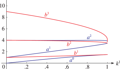
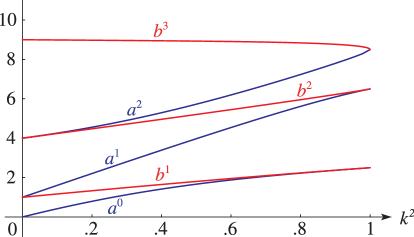
►They are denoted by , , , , where ; see Table 29.3.1.
…
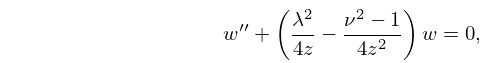
►The quantity satisfies equation (29.3.10) with
…
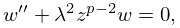
►The quantity satisfies equation (29.3.10) with
…
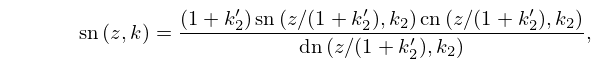
►The quantity satisfies equation (29.3.10) with
…
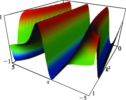
►The eigenfunctions corresponding to the eigenvalues of §29.3(i) are denoted by , , , .
…
 ►
►
 ►
►
 ►
►
 ►
►
 ►
►
