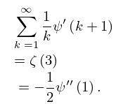
About the Project

赞恩州立学院国际商务文凭证书〖办证V信ATV1819〗psiup

AdvancedHelp

(0.002 seconds)

1—10 of 100 matching pages

1: 5.15 Polygamma Functions
The functions ψ ( n ) ( z ) , n = 1 , 2 , , are called the polygamma functions. In particular, ψ ( z ) is the trigamma function; ψ ′′ , ψ ( 3 ) , ψ ( 4 ) are the tetra-, penta-, and hexagamma functions respectively. …
5.15.5 ψ ( n ) ( z + 1 ) = ψ ( n ) ( z ) + ( 1 ) n n ! z n 1 ,
5.15.7 ψ ( n ) ( m z ) = 1 m n + 1 k = 0 m 1 ψ ( n ) ( z + k m ) .
For continued fractions for ψ ( z ) and ψ ′′ ( z ) see Cuyt et al. (2008, pp. 231–238).
2: 5.16 Sums
5.16.1 k = 1 ( 1 ) k ψ ( k ) = π 2 8 ,
5.16.2 k = 1 1 k ψ ( k + 1 ) = ζ ( 3 ) = 1 2 ψ ′′ ( 1 ) .
3: 4.12 Generalized Logarithms and Exponentials
Its inverse ψ ( x ) is called a generalized logarithm. It, too, is strictly increasing when 0 x 1 , and
4.12.3 ψ ( e x ) = 1 + ψ ( x ) , < x < ,
4.12.4 ψ ( 0 ) = 0 .
Both ϕ ( x ) and ψ ( x ) are continuously differentiable. …
4: 36.10 Differential Equations
§36.10(i) Equations for Ψ K ( 𝐱 )
In terms of the normal form (36.2.1) the Ψ K ( 𝐱 ) satisfy the operator equation … In terms of the normal forms (36.2.2) and (36.2.3), the Ψ ( U ) ( 𝐱 ) satisfy the following operator equations …
5: 36.3 Visualizations of Canonical Integrals
Figure 36.3.1: Modulus of Pearcey integral | Ψ 2 ( x , y ) | . …
Figure 36.3.2: Modulus of swallowtail canonical integral function | Ψ 3 ( x , y , 3 ) | . …
In Figure 36.3.13(a) points of confluence of phase contours are zeros of Ψ 2 ( x , y ) ; similarly for other contour plots in this subsection. In Figure 36.3.13(b) points of confluence of all colors are zeros of Ψ 2 ( x , y ) ; similarly for other density plots in this subsection.
Figure 36.3.13: Phase of Pearcey integral ph Ψ 2 ( x , y ) . …
6: 5.1 Special Notation
The main functions treated in this chapter are the gamma function Γ ( z ) , the psi function (or digamma function) ψ ( z ) , the beta function B ( a , b ) , and the q -gamma function Γ q ( z ) . … Alternative notations for the psi function are: Ψ ( z 1 ) (Gauss) Jahnke and Emde (1945); Ψ ( z ) Davis (1933); 𝖥 ( z 1 ) Pairman (1919). …
7: 5.24 Software
§5.24(iii) ψ ( x ) , ψ ( n ) ( x ) , x
§5.24(iv) Γ ( z ) , ψ ( z ) , ψ ( n ) ( z ) , z
8: 19.11 Addition Theorems
In the case of θ , ϕ [ 0 , π / 2 ) and 0 k 2 α 2 < min ( 1 , ( 1 cos θ cos ϕ cos ψ ) 1 ) , we can use …
§19.11(ii) Case ψ = π / 2
sin θ = ( sin ψ ) / ( 1 + cos ψ ) ( 1 + Δ ( ψ ) ) ,
cos θ = ( cos ψ ) + Δ ( ψ ) 1 + Δ ( ψ ) ,
tan θ = tan ( 1 2 ψ ) 1 + cos ψ ( cos ψ ) + Δ ( ψ ) ,
9: 5.22 Tables
Abramowitz and Stegun (1964, Chapter 6) tabulates Γ ( x ) , ln Γ ( x ) , ψ ( x ) , and ψ ( x ) for x = 1 ( .005 ) 2 to 10D; ψ ′′ ( x ) and ψ ( 3 ) ( x ) for x = 1 ( .01 ) 2 to 10D; Γ ( n ) , 1 / Γ ( n ) , Γ ( n + 1 2 ) , ψ ( n ) , log 10 Γ ( n ) , log 10 Γ ( n + 1 3 ) , log 10 Γ ( n + 1 2 ) , and log 10 Γ ( n + 2 3 ) for n = 1 ( 1 ) 101 to 8–11S; Γ ( n + 1 ) for n = 100 ( 100 ) 1000 to 20S. Zhang and Jin (1996, pp. 67–69 and 72) tabulates Γ ( x ) , 1 / Γ ( x ) , Γ ( x ) , ln Γ ( x ) , ψ ( x ) , ψ ( x ) , ψ ( x ) , and ψ ( x ) for x = 0 ( .1 ) 5 to 8D or 8S; Γ ( n + 1 ) for n = 0 ( 1 ) 100 ( 10 ) 250 ( 50 ) 500 ( 100 ) 3000 to 51S. … This reference also includes ψ ( x + i y ) for the same arguments to 5D. Zhang and Jin (1996, pp. 70, 71, and 73) tabulates the real and imaginary parts of Γ ( x + i y ) , ln Γ ( x + i y ) , and ψ ( x + i y ) for x = 0.5 , 1 , 5 , 10 , y = 0 ( .5 ) 10 to 8S.
10: 36.1 Special Notation
The main functions covered in this chapter are cuspoid catastrophes Φ K ( t ; 𝐱 ) ; umbilic catastrophes with codimension three Φ ( E ) ( s , t ; 𝐱 ) , Φ ( H ) ( s , t ; 𝐱 ) ; canonical integrals Ψ K ( 𝐱 ) , Ψ ( E ) ( 𝐱 ) , Ψ ( H ) ( 𝐱 ) ; diffraction catastrophes Ψ K ( 𝐱 ; k ) , Ψ ( E ) ( 𝐱 ; k ) , Ψ ( H ) ( 𝐱 ; k ) generated by the catastrophes. …