%E4%BA%9A%E6%B4%B2%E5%8D%9A%E5%BD%A9%E5%B9%B3%E5%8F%B0,%E4%BA%9A%E6%B4%B2%E5%8D%9A%E5%BD%A9%E5%85%AC%E5%8F%B8,%E3%80%90%E4%BA%9A%E6%B4%B2%E5%8D%9A%E5%BD%A9%E7%BD%91%E5%9D%80%E2%88%B622kk33.com%E3%80%91%E4%BD%93%E8%82%B2%E5%8D%9A%E5%BD%A9%E5%85%AC%E5%8F%B8%E6%8E%92%E5%90%8D,%E6%9C%80%E5%A4%A7%E7%9A%84%E5%8D%9A%E5%BD%A9%E5%85%AC%E5%8F%B8,%E4%BA%9A%E6%B4%B2%E4%BD%93%E8%82%B2%E5%8D%9A%E5%BD%A9%E5%B9%B3%E5%8F%B0%E3%80%90%E7%BA%BF%E4%B8%8A%E5%8D%9A%E5%BD%A9%E2%88%B622kk33.com%E3%80%91%E7%BD%91%E5%9D%80ZEkEnBDkCBgfk0kC

SearchAdvancedHelp

(0.057 seconds)

21—30 of 601 matching pages

21: 10 Bessel Functions

…

22: 23 Weierstrass Elliptic and Modular
Functions

…

23: 26.5 Lattice Paths: Catalan Numbers

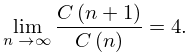
… ► $C\left(n\right)$ is the Catalan number. …(Sixty-six equivalent definitions of $C\left(n\right)$ are given in Stanley (1999, pp. 219–229).) … ►

26.5.3 $$C\left(n+1\right)=\sum _{k=0}^{n}C\left(k\right)C\left(n-k\right),$$

ⓘ

Symbols:

$C\left(n\right)$: Catalan number, $k$: nonnegative integer and $n$: nonnegative integer

Permalink:

http://dlmf.nist.gov/26.5.E3

Encodings:

pMML, png, TeX

See also:

Annotations for §26.5(iii), §26.5 and Ch.26

►

26.5.4 $$C\left(n+1\right)=\frac{2(2n+1)}{n+2}C\left(n\right),$$

ⓘ

Symbols:

$C\left(n\right)$: Catalan number and $n$: nonnegative integer

Permalink:

http://dlmf.nist.gov/26.5.E4

Encodings:

pMML, png, TeX

See also:

Annotations for §26.5(iii), §26.5 and Ch.26

… ►

26.5.7 $$\underset{n\to \mathrm{\infty }}{lim}\frac{C\left(n+1\right)}{C\left(n\right)}=4.$$

ⓘ

Symbols:

$C\left(n\right)$: Catalan number and $n$: nonnegative integer

Permalink:

http://dlmf.nist.gov/26.5.E7

Encodings:

pMML, png, TeX

See also:

Annotations for §26.5(iv), §26.5 and Ch.26

24: 3.4 Differentiation

… ►where $A_k^n$ is as in (3.3.10). … ►

$$B_{-2}^6=\frac{1}{60}(9-9t-30t^2+20t^3+5t^4-3t^5),$$

… ►

$$B_2^6=-\frac{1}{60}(9+9t-30t^2-20t^3+5t^4+3t^5),$$

… ►where $C$ is a simple closed contour described in the positive rotational sense such that $C$ and its interior lie in the domain of analyticity of $f$, and $x_0$ is interior to $C$. Taking $C$ to be a circle of radius $r$ centered at $x_0$, we obtain …

25: 14.33 Tables

… ►

Abramowitz and Stegun (1964, Chapter 8) tabulates ${𝖯}_n\left(x\right)$ for $n=0(1)3,9,10$, $x=0(.01)1$, 5–8D; ${𝖯}_n^{\prime }\left(x\right)$ for $n=1(1)4,9,10$, $x=0(.01)1$, 5–7D; ${𝖰}_n\left(x\right)$ and ${𝖰}_n^{\prime }\left(x\right)$ for $n=0(1)3,9,10$, $x=0(.01)1$, 6–8D; $P_n\left(x\right)$ and $P_n^{\prime }\left(x\right)$ for $n=0(1)5,9,10$, $x=1(.2)10$, 6S; $Q_n\left(x\right)$ and $Q_n^{\prime }\left(x\right)$ for $n=0(1)3,9,10$, $x=1(.2)10$, 6S. (Here primes denote derivatives with respect to $x$.)

►

Zhang and Jin (1996, Chapter 4) tabulates ${𝖯}_n\left(x\right)$ for $n=2(1)5,10$, $x=0(.1)1$, 7D; ${𝖯}_n\left(\cos \theta \right)$ for $n=1(1)4,10$, $\theta =0(5^{\circ }){90}^{\circ }$, 8D; ${𝖰}_n\left(x\right)$ for $n=0(1)2,10$, $x=0(.1)0.9$, 8S; ${𝖰}_n\left(\cos \theta \right)$ for $n=0(1)3,10$, $\theta =0(5^{\circ }){90}^{\circ }$, 8D; ${𝖯}_n^m\left(x\right)$ for $m=1(1)4$, $n-m=0(1)2$, $n=10$, $x=0,0.5$, 8S; ${𝖰}_n^m\left(x\right)$ for $m=1(1)4$, $n=0(1)2,10$, 8S; ${𝖯}_{\nu }^m\left(\cos \theta \right)$ for $m=0(1)3$, $\nu =0(.25)5$, $\theta =0({15}^{\circ }){90}^{\circ }$, 5D; $P_n\left(x\right)$ for $n=2(1)5,10$, $x=1(1)10$, 7S; $Q_n\left(x\right)$ for $n=0(1)2,10$, $x=2(1)10$, 8S. Corresponding values of the derivative of each function are also included, as are 6D values of the first 5 $\nu$-zeros of ${𝖯}_{\nu }^m\left(\cos \theta \right)$ and of its derivative for $m=0(1)4$, $\theta ={10}^{\circ },{30}^{\circ },{150}^{\circ }$.

►

Belousov (1962) tabulates ${𝖯}_n^m\left(\cos \theta \right)$ (normalized) for $m=0(1)36$, $n-m=0(1)56$, $\theta =0({2.5}^{\circ }){90}^{\circ }$, 6D.

…

26: 16.7 Relations to Other Functions

… ►For $\mathit{3}j$, $\mathit{6}j$, $\mathit{9}j$ symbols see Chapter 34. Further representations of special functions in terms of ${}_p{}^{}F_q^{}$ functions are given in Luke (1969a, §§6.2–6.3), and an extensive list of ${}_{q+1}{}^{}F_q^{}$ functions with rational numbers as parameters is given in Krupnikov and Kölbig (1997).

27: 34.8 Approximations for Large Parameters

§34.8 Approximations for Large Parameters

►For large values of the parameters in the $\mathit{3}j$, $\mathit{6}j$, and $\mathit{9}j$ symbols, different asymptotic forms are obtained depending on which parameters are large. … ►For approximations for the $\mathit{3}j$, $\mathit{6}j$, and $\mathit{9}j$ symbols with error bounds see Flude (1998), Chen et al. (1999), and Watson (1999): these references also cite earlier work.

28: 1.11 Zeros of Polynomials

… ►Set $z=w-\frac{1}{3}a$ to reduce $f(z)=z^3+a{z}^2+bz+c$ to $g(w)=w^3+pw+q$, with $p=(3b-a^2)/3$, $q=(2a^3-9ab+27c)/27$. … ► $f(z)=z^3-6z^2+6z-2$, $g(w)=w^3-6w-6$, $A=3\sqrt[3]{4}$, $B=3\sqrt[3]{2}$. … ►Resolvent cubic is $z^3+12z^2+20z+9=0$ with roots ${\theta }_1=-1$, ${\theta }_2=-\frac{1}{2}(11+\sqrt{85})$, ${\theta }_3=-\frac{1}{2}(11-\sqrt{85})$, and $\sqrt{-{\theta }_1}=1$, $\sqrt{-{\theta }_2}=\frac{1}{2}(\sqrt{17}+\sqrt{5})$, $\sqrt{-{\theta }_3}=\frac{1}{2}(\sqrt{17}-\sqrt{5})$. … ►Let … ►Then $f(z)$, with $a_n\ne 0$, is stable iff $a_0\ne 0$; $D_{2k}>0$, $k=1,\mathrm{\dots },\lfloor \frac{1}{2}n\rfloor$; $\mathrm{sign}{D}_{2k+1}=\mathrm{sign}{a}_0$, $k=0,1,\mathrm{\dots },\lfloor \frac{1}{2}n-\frac{1}{2}\rfloor$.

29: 18.8 Differential Equations

… ►

Table 18.8.1: Classical OP’s: differential equations $A(x)f^{\prime \prime }(x)+B(x)f^{\prime }(x)+C(x)f(x)+{\lambda }_{n}f(x)=0$.

► ►►►►►

#	$f(x)$	$A(x)$	$B(x)$	$C(x)$	${\lambda }_n$
…
4	$C_n^{(\lambda )}\left(x\right)$	$1-x^2$	$-(2\lambda +1)x$	$0$	$n(n+2\lambda )$
…
8	$L_n^{(\alpha )}\left(x\right)$	$x$	$\alpha +1-x$	$0$	$n$
9	${\mathrm{e}}^{-\frac{1}{2}{x}^2}{x}^{\alpha +\frac{1}{2}}{L}_n^{(\alpha )}\left(x^2\right)$	$1$	$0$	$-x^2+(\frac{1}{4}-{\alpha }^2)x^{-2}$	$4n+2\alpha +2$
…

►

…

30: Bibliography

… ►

Evaluation of Coulomb wave functions along the transition line. Physical Rev. (2) 96, pp. 77–79.

ⓘ

External Links:

Document, MathReview (A. Erdélyi), ZentralBlatt

Referenced by:

§33.12(i).

Encodings:

BibTeX

… ►

Algorithm 610. A portable FORTRAN subroutine for derivatives of the psi function. ACM Trans. Math. Software 9 (4), pp. 494–502.

ⓘ

Notes:

Single and double precision, maximum accuracy 18S.

External Links:

ISSN 0098-3500, Document, GAMS (module 610; package TOMS), MathReview Entry, ZentralBlatt

Referenced by:

1st item.

Encodings:

BibTeX

… ►

Theorems on generalized Dedekind sums. Pacific J. Math. 2 (1), pp. 1–9.

ⓘ

External Links:

MathReview (N. G. de Bruijn), ZentralBlatt

Referenced by:

(25.11.41), (25.11.42), §25.11(xii).

Encodings:

BibTeX

… ►

Numerical Tables for Angular Correlation Computations in $\alpha$-, $\beta$- and $\gamma$-Spectroscopy: $3j$-, $6j$-, $9j$-Symbols, F- and $\mathrm{\Gamma }$-Coefficients. Landolt-Börnstein Numerical Data and Functional Relationships in Science and Technology, Springer-Verlag.

ⓘ

External Links:

ISBN 978-3-540-04218-1

Referenced by:

§34.14.

Encodings:

BibTeX

… ►

A new treatment of the ellipsoidal wave equation. Proc. London Math. Soc. (3) 9, pp. 21–50.

ⓘ

External Links:

ISSN 0024-6115, Document, MathReview (J. Meixner), ZentralBlatt

Referenced by:

§29.11.

Encodings:

BibTeX

…