visualizations of modulus

SearchAdvancedHelp

(0.001 seconds)

6 matching pages

1: 36.3 Visualizations of Canonical Integrals

… ►

§36.3(i) Canonical Integrals: Modulus

… ►

…

Figure 36.3.12: Modulus of hyperbolic umbilic canonical integral function $|{\mathrm{\Psi }}^{(\mathrm{H})}\left(x,y,3\right)|$. …

…

2: 36.5 Stokes Sets

… ►The Stokes set consists of the rays $\mathrm{ph}x=\pm 2\pi /3$ in the complex $x$-plane. … ►For , there are two solutions $u$, provided that $|Y|>{(\frac{2}{5})}^{1/2}$. … ►This consists of three separate cusp-edged sheets connected to the cusp-edged sheets of the bifurcation set, and related by rotation about the $z$-axis by $2\pi /3$. … ►

§36.5(iv) Visualizations

… ►

►►

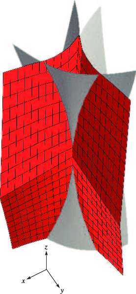
Figure 36.5.9: Sheets of the Stokes surface for the hyperbolic umbilic catastrophe (colored and with mesh) and the bifurcation set (gray). Magnify

3: 9.9 Zeros

… ►They lie in the sectors and , and are denoted by ${\beta }_k$, ${\beta }_k^{\prime }$, respectively, in the former sector, and by $\overline{{\beta }_k}$, $\overline{{\beta }_k^{\prime }}$, in the conjugate sector, again arranged in ascending order of absolute value (modulus) for $k=1,2,\mathrm{\dots }.$ See §9.3(ii) for visualizations. …

4: 28.33 Physical Applications

… ►with $W(x,y,t)={\mathrm{e}}^{\mathrm{i}\omega t}V(x,y)$, reduces to (28.32.2) with $k^2={\omega }^2\rho /\tau$. …If we denote the positive solutions $q$ of (28.33.3) by $q_{n,m}$, then the vibration of the membrane is given by ${\omega }_{n,m}^2=4q_{n,m}\tau /(c^2\rho )$. … ►For a visualization see Gutiérrez-Vega et al. (2003), and for references to other boundary-value problems see: … ►Substituting $z=\omega t$, $a=b/{\omega }^2$, and $2q=f/{\omega }^2$, we obtain Mathieu’s standard form (28.2.1). ►As $\omega$ runs from $0$ to $+\mathrm{\infty }$, with $b$ and $f$ fixed, the point $(q,a)$ moves from $\mathrm{\infty }$ to $0$ along the ray $ℒ$ given by the part of the line $a=(2b/f)q$ that lies in the first quadrant of the $(q,a)$-plane. …

5: Errata

… ►

Scales were corrected in all figures. The interval $-8.4\le \frac{x-y}{\sqrt{2}}\le 8.4$ was replaced by $-12.0\le \frac{x-y}{\sqrt{2}}\le 12.0$ and $-12.7\le \frac{x+y}{\sqrt{2}}\le 4.2$ replaced by $-18.0\le \frac{x+y}{\sqrt{2}}\le 6.0$. All plots and interactive visualizations were regenerated to improve image quality.

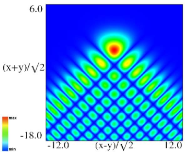
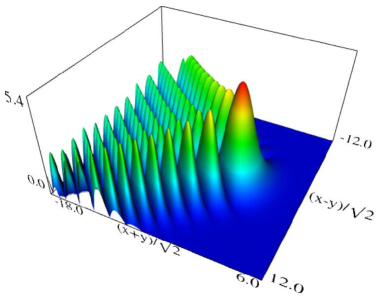
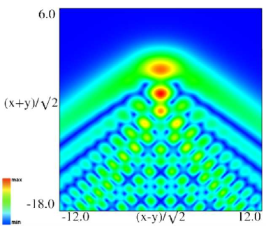
(a) Density plot.	(b) 3D plot.

Figure 36.3.9: Modulus of hyperbolic umbilic canonical integral function $|{\mathrm{\Psi }}^{(\mathrm{H})}\left(x,y,0\right)|$.

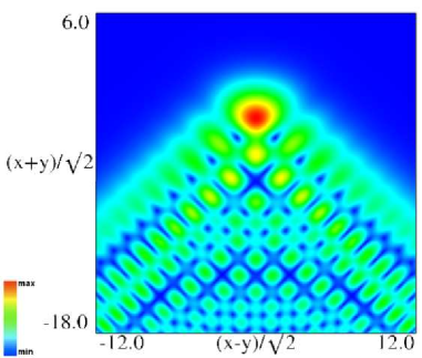
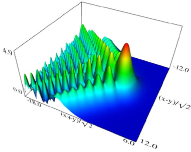
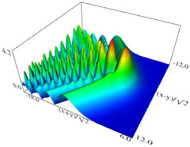
(a) Density plot.	(b) 3D plot.

Figure 36.3.10: Modulus of hyperbolic umbilic canonical integral function $|{\mathrm{\Psi }}^{(\mathrm{H})}\left(x,y,1\right)|$.

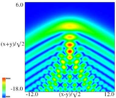
(a) Density plot.	(b) 3D plot.

Figure 36.3.11: Modulus of hyperbolic umbilic canonical integral function $|{\mathrm{\Psi }}^{(\mathrm{H})}\left(x,y,2\right)|$.

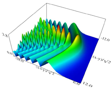
(a) Density plot.	(b) 3D plot.

Figure 36.3.12: Modulus of hyperbolic umbilic canonical integral function $|{\mathrm{\Psi }}^{(\mathrm{H})}\left(x,y,3\right)|$.

Reported 2016-09-12 by Dan Piponi.

…

6: About Color Map

… ►Surface visualizations in the DLMF represent functions of the form $z=f(x,y)$ by the height $z$ or the magnitude, $|z|$, for complex functions, over the $x\times y$ plane. … ►In doing this, however, we would like to place the mathematically significant phase values, specifically the multiples of $\pi /2$ correponding to the real and imaginary axes, at more immediately recognizable colors. … ►We therefore use a piecewise linear mapping as illustrated below, that takes phase $0$ to red, $\pi /2$ to yellow, $\pi$ to cyan and $3\pi /2$ to blue. …