turning points

SearchAdvancedHelp

(0.002 seconds)

1—10 of 24 matching pages

1: 33.23 Methods of Computation

… ►Inside the turning points, that is, when , there can be a loss of precision by a factor of approximately ${|G_{\mathrm{\ell }}|}^2$. … ►WKBJ approximations (§2.7(iii)) for $\rho >{\rho }_{\mathrm{tp}}(\eta ,\mathrm{\ell })$ are presented in Hull and Breit (1959) and Seaton and Peach (1962: in Eq. … ►Hull and Breit (1959) and Barnett (1981b) give WKBJ approximations for $F_0$ and $G_0$ in the region inside the turning point: .

2: 33.3 Graphics

… ►

►►

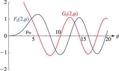
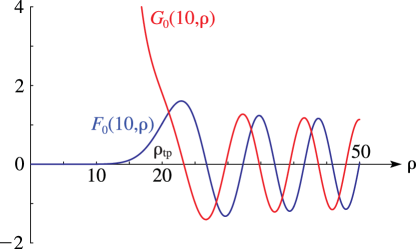
Figure 33.3.3: $F_{\mathrm{\ell }}(\eta ,\rho )$, $G_{\mathrm{\ell }}(\eta ,\rho )$ with $\mathrm{\ell }=0$, $\eta =2$. The turning point is at ${\rho }_{\mathrm{tp}}(2,0)=4$. Magnify

►

►►

Figure 33.3.4: $F_{\mathrm{\ell }}(\eta ,\rho )$, $G_{\mathrm{\ell }}(\eta ,\rho )$ with $\mathrm{\ell }=0$, $\eta =10$. The turning point is at ${\rho }_{\mathrm{tp}}(10,0)=20$. Magnify

… ►

►►

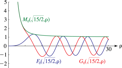
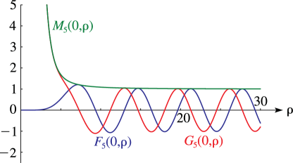
Figure 33.3.5: $F_{\mathrm{\ell }}(\eta ,\rho )$, $G_{\mathrm{\ell }}(\eta ,\rho )$, and $M_{\mathrm{\ell }}(\eta ,\rho )$ with $\mathrm{\ell }=0$, $\eta =\sqrt{15/2}$. The turning point is at ${\rho }_{\mathrm{tp}}(\sqrt{15/2},0)=\sqrt{30}=5.47\mathrm{\dots }$. Magnify

►

►►

Figure 33.3.6: $F_{\mathrm{\ell }}(\eta ,\rho )$, $G_{\mathrm{\ell }}(\eta ,\rho )$, and $M_{\mathrm{\ell }}(\eta ,\rho )$ with $\mathrm{\ell }=5$, $\eta =0$. The turning point is at ${\rho }_{\mathrm{tp}}(0,5)=\sqrt{30}$ (as in Figure 33.3.5). Magnify

…

3: 9.15 Mathematical Applications

… ►Airy functions play an indispensable role in the construction of uniform asymptotic expansions for contour integrals with coalescing saddle points, and for solutions of linear second-order ordinary differential equations with a simple turning point. …

4: 33.14 Definitions and Basic Properties

… ►

§33.14(i) Coulomb Wave Equation

… ►When $ϵ>0$ the outer turning point is given by ►

33.14.3 $$r_{\mathrm{tp}}(ϵ,\mathrm{\ell })=\left(\sqrt{1+ϵ\mathrm{\ell }(\mathrm{\ell }+1)}-1\right)/ϵ;$$

ⓘ

Defines:

$r_{\mathrm{tp}}(ϵ,\mathrm{\ell })$: outer turning point for Coulomb functions

Symbols:

$\mathrm{\ell }$: nonnegative integer and $ϵ$: real parameter

Permalink:

http://dlmf.nist.gov/33.14.E3

Encodings:

pMML, png, TeX

See also:

Annotations for §33.14(i), §33.14 and Ch.33

…

5: 33.2 Definitions and Basic Properties

… ►

§33.2(i) Coulomb Wave Equation

… ►There are two turning points, that is, points at which $d^{2}w/{d\rho }^2=0$ (§2.8(i)). … ►

33.2.2 $${\rho }_{\mathrm{tp}}(\eta ,\mathrm{\ell })=\eta +{({\eta }^2+\mathrm{\ell }(\mathrm{\ell }+1))}^{1/2}.$$

ⓘ

Defines:

${\rho }_{\mathrm{tp}}(\eta ,\mathrm{\ell })$: outer turning point for Coulomb radial functions

Symbols:

$\mathrm{\ell }$: nonnegative integer and $\eta$: real parameter

Referenced by:

§33.12(i), §33.14(i)

Permalink:

http://dlmf.nist.gov/33.2.E2

Encodings:

pMML, png, TeX

See also:

Annotations for §33.2(i), §33.2 and Ch.33

…

6: 10.72 Mathematical Applications

… ►

§10.72(i) Differential Equations with Turning Points

… ►

Simple Turning Points

… ►These expansions are uniform with respect to $z$, including the turning point $z_0$ and its neighborhood, and the region of validity often includes cut neighborhoods (§1.10(vi)) of other singularities of the differential equation, especially irregular singularities. … ►

Multiple or Fractional Turning Points

… ►

§10.72(iii) Differential Equations with a Double Pole and a Movable Turning Point

…

7: 12.16 Mathematical Applications

… ►PCFs are used as basic approximating functions in the theory of contour integrals with a coalescing saddle point and an algebraic singularity, and in the theory of differential equations with two coalescing turning points; see §§2.4(vi) and 2.8(vi). …

8: 13.27 Mathematical Applications

… ►For applications of Whittaker functions to the uniform asymptotic theory of differential equations with a coalescing turning point and simple pole see §§2.8(vi) and 18.15(i). …

9: 9.16 Physical Applications

… ►The frequent appearances of the Airy functions in both classical and quantum physics is associated with wave equations with turning points, for which asymptotic (WKBJ) solutions are exponential on one side and oscillatory on the other. The Airy functions constitute uniform approximations whose region of validity includes the turning point and its neighborhood. … ►This reference provides several examples of applications to problems in quantum mechanics in which Airy functions give uniform asymptotic approximations, valid in the neighborhood of a turning point. …

10: 33.12 Asymptotic Expansions for Large $\eta$

… ►When $\mathrm{\ell }=0$ and $\eta >0$, the outer turning point is given by ${\rho }_{\mathrm{tp}}(\eta ,0)=2\eta$; compare (33.2.2). …