sums of squares
(0.002 seconds)
41—48 of 48 matching pages
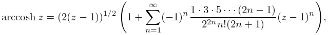
41: 4.38 Inverse Hyperbolic Functions: Further Properties
…
►
4.38.4
, .
…
►In the following equations square roots have their principal values.
…
►All square roots have either possible value.
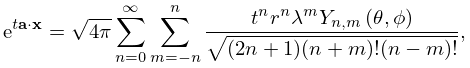
42: 14.30 Spherical and Spheroidal Harmonics
…
►
14.30.8_5
…
►
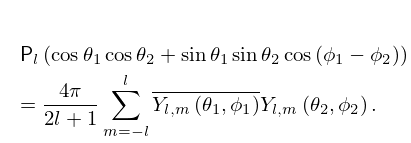
§14.30(iii) Sums
… ►
14.30.9
…
►Here, in spherical coordinates, is the squared angular momentum operator:
…
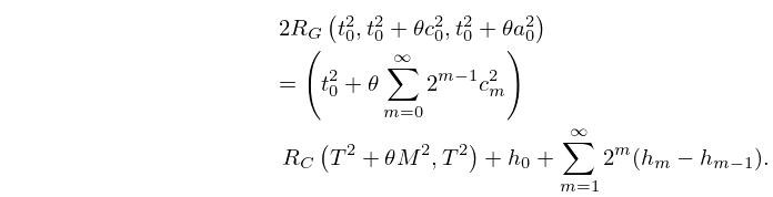
43: 19.36 Methods of Computation
…
►When the differences are moderately small, the iteration is stopped, the elementary symmetric functions of certain differences are calculated, and a polynomial consisting of a fixed number of terms of the sum in (19.19.7) is evaluated.
…
►The reductions in §19.29(i) represent as squares, for example in (19.29.4).
…
►
19.36.13
…
44: 8.12 Uniform Asymptotic Expansions for Large Parameter
…
►where the branch of the square root is continuous and satisfies as .
…
►
8.12.7
…
►
8.12.11
,
…
►
8.12.13
.
…
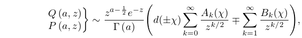
►
8.12.18
…
45: 4.45 Methods of Computation
…
►Then we take square roots repeatedly until is sufficiently small, where
…
►Another method, when is large, is to sum
…
46: 19.20 Special Cases
47: 19.29 Reduction of General Elliptic Integrals
…
►These theorems reduce integrals over a real interval of certain integrands containing the square root of a quartic or cubic polynomial to symmetric integrals over containing the square root of a cubic polynomial (compare §19.16(i)).
…
►
19.29.12
…
►The only cases that are integrals of the third kind are those in which at least one with is a negative integer and those in which and is a positive integer.
…
►
19.29.18
;
…
►If both square roots in (19.29.22) are 0, then the indeterminacy in the two preceding equations can be removed by using (19.27.8) to evaluate the integral as multiplied either by or by in the cases of (19.29.20) or (19.29.21), respectively.
…
