reduced%20residue%20system

(0.002 seconds)

11—20 of 231 matching pages

11: 19.36 Methods of Computation

… ►Numerical differences between the variables of a symmetric integral can be reduced in magnitude by successive factors of 4 by repeated applications of the duplication theorem, as shown by (19.26.18). … ►The incomplete integrals

R_{F}\left(x,y,z\right)

and

R_{G}\left(x,y,z\right)

can be computed by successive transformations in which two of the three variables converge quadratically to a common value and the integrals reduce to

R_{C}

, accompanied by two quadratically convergent series in the case of

R_{G}

; compare Carlson (1965, §§5,6). …If

t_{0}=a_{0}

and

\theta=-1

, so that

t_{n}=a_{n}

, then this procedure reduces to the AGM method for the complete integral. … ►(19.22.20) reduces to

0=0

p=x

p=y

, and (19.22.19) reduces to

0=0

z=x

z=y

. … ►For computation of Legendre’s integral of the third kind, see Abramowitz and Stegun (1964, §§17.7 and 17.8, Examples 15, 17, 19, and 20). …

12: 8 Incomplete Gamma and Related
Functions

…

13: 28 Mathieu Functions and Hill’s Equation

…

14: 8.26 Tables

… ►

•

Khamis (1965) tabulates $P\left(a,x\right)$ for $a=0.05(.05)10(.1)20(.25)70$ , $0.0001\leq x\leq 250$ to 10D.

… ►

•

Abramowitz and Stegun (1964, pp. 245–248) tabulates $E_{n}\left(x\right)$ for $n=2,3,4,10,20$ , $x=0(.01)2$ to 7D; also $(x+n)e^{x}E_{n}\left(x\right)$ for $n=2,3,4,10,20$ , $x^{-1}=0(.01)0.1(.05)0.5$ to 6S.

… ►

•

Pagurova (1961) tabulates $E_{n}\left(x\right)$ for $n=0(1)20$ , $x=0(.01)2(.1)10$ to 4-9S; $e^{x}E_{n}\left(x\right)$ for $n=2(1)10$ , $x=10(.1)20$ to 7D; $e^{x}E_{p}\left(x\right)$ for $p=0(.1)1$ , $x=0.01(.01)7(.05)12(.1)20$ to 7S or 7D.

… ►

•

Zhang and Jin (1996, Table 19.1) tabulates $E_{n}\left(x\right)$ for $n=1,2,3,5,10,15,20$ , $x=0(.1)1,1.5,2,3,5,10,20,30,50,100$ to 7D or 8S.

15: 23 Weierstrass Elliptic and Modular
Functions

…

16: 36 Integrals with Coalescing Saddles

…

17: Gergő Nemes

… ►As of September 20, 2021, Nemes performed a complete analysis and acted as main consultant for the update of the source citation and proof metadata for every formula in Chapter 25 Zeta and Related Functions. …

18: 33.24 Tables

… ►

•

Abramowitz and Stegun (1964, Chapter 14) tabulates $F_{0}\left(\eta,\rho\right)$ , $G_{0}\left(\eta,\rho\right)$ , $F_{0}'\left(\eta,\rho\right)$ , and $G_{0}'\left(\eta,\rho\right)$ for $\eta=0.5(.5)20$ and $\rho=1(1)20$ , 5S; $C_{0}\left(\eta\right)$ for $\eta=0(.05)3$ , 6S.

…

19: 25.11 Hurwitz Zeta Function

… ►

\zeta\left(s,a\right)

has a meromorphic continuation in the

s

-plane, its only singularity in

\mathbb{C}

being a simple pole at

s=1

with residue

1

. … ►

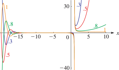
See accompanying text — Figure 25.11.1: Hurwitz zeta function $\zeta\left(x,a\right)$ , $a$ = 0. …8, 1, $-20\leq x\leq 10$ . … Magnify

… ►When

a=\frac{1}{2}

, (25.11.10) reduces to (25.8.3); compare (25.11.11). … ►When

a=1

, (25.11.35) reduces to (25.2.3). …

20: Bibliography D

… ►

C. de la Vallée Poussin (1896a) Recherches analytiques sur la théorie des nombres premiers. Première partie. La fonction

\zeta(s)

de Riemann et les nombres premiers en général, suivi d’un Appendice sur des réflexions applicables à une formule donnée par Riemann. Ann. Soc. Sci. Bruxelles 20, pp. 183–256 (French).

ⓘ

Notes:: Reprinted in Collected works/Oeuvres scientifiques, Vol. I, pp. 223–296 Académie Royale de Belgique, Brussels, 2000.
External Links:: MathReview, ZentralBlatt
Referenced by:: §25.10(i), §27.11, §27.2(i).
Encodings:: BibTeX

►

C. de la Vallée Poussin (1896b) Recherches analytiques sur la théorie des nombres premiers. Deuxième partie. Les fonctions de Dirichlet et les nombres premiers de la forme linéaire

Mx+N

. Ann. Soc. Sci. Bruxelles 20, pp. 281–397 (French).

ⓘ

Notes:: Reprinted in Collected works/Oeuvres scientifiques, Vol. I, pp. 309–425, Académie Royale de Belgique, Brussels, 2000.
External Links:: MathReview, ZentralBlatt
Referenced by:: §25.10(i), §27.11, §27.2(i).
Encodings:: BibTeX

… ►

K. Dilcher (1987b) Irreducibility of certain generalized Bernoulli polynomials belonging to quadratic residue class characters. J. Number Theory 25 (1), pp. 72–80.

ⓘ

External Links:: ISSN 0022-314X, Document, MathReview (T. Metsänkylä)
Referenced by:: §24.12(iii).
Encodings:: BibTeX

… ►

B. Döring (1966) Complex zeros of cylinder functions. Math. Comp. 20 (94), pp. 215–222.

ⓘ

Notes:: For a numerical error in one of the zeros see Amos (1985).
External Links:: ISSN 0025-5718, FullText, MathReview, ZentralBlatt
Referenced by:: 2nd item.
Encodings:: BibTeX

… ►

T. M. Dunster (1989) Uniform asymptotic expansions for Whittaker’s confluent hypergeometric functions. SIAM J. Math. Anal. 20 (3), pp. 744–760.

ⓘ

Notes:: (This reference has several typographical errors.)
External Links:: ISSN 0036-1410, Document, MathReview (F. W. J. Olver), ZentralBlatt
Referenced by:: §13.21(ii), §13.21(iii), §13.21(iv).
Encodings:: BibTeX

…