q-multinomial%20coefficient

SearchAdvancedHelp

(0.002 seconds)

11—20 of 293 matching pages

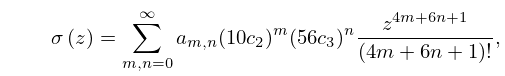
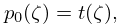
11: 23.9 Laurent and Other Power Series

… ►

$c_2={\displaystyle \frac{1}{20}}{g}_2,$

… ►Explicit coefficients $c_n$ in terms of $c_2$ and $c_3$ are given up to $c_{19}$ in Abramowitz and Stegun (1964, p. 636). … ►

23.9.7 $$\sigma \left(z\right)=\sum _{m,n=0}^{\mathrm{\infty }}{a}_{m,n}{(10c_2)}^m{(56c_3)}^n\frac{z^{4m+6n+1}}{(4m+6n+1)!},$$

ⓘ

Symbols:

$\sigma \left(z\right)$ (= $\sigma \left(z|𝕃\right)$ = $\sigma (z;g_2,g_3)$): Weierstrass sigma function, $!$: factorial (as in $n!$), $𝕃$: lattice, $n$: integer, $m$: integer, $z$: complex, $c_n$ and $a_{m,n}$: coefficients

A&S Ref:

18.5.6

Referenced by:

§23.9

Permalink:

http://dlmf.nist.gov/23.9.E7

Encodings:

pMML, png, TeX

See also:

Annotations for §23.9 and Ch.23

►where $a_{0,0}=1$, $a_{m,n}=0$ if either $m$ or , and ►

23.9.8 $$a_{m,n}=3(m+1)a_{m+1,n-1}+\frac{16}{3}(n+1)a_{m-2,n+1}-\frac{1}{3}(2m+3n-1)(4m+6n-1)a_{m-1,n}.$$

ⓘ

Symbols:

$n$: integer, $m$: integer and $a_{m,n}$: coefficients

A&S Ref:

18.5.8

Permalink:

http://dlmf.nist.gov/23.9.E8

Encodings:

pMML, png, TeX

See also:

Annotations for §23.9 and Ch.23

…

12: 8 Incomplete Gamma and Related
Functions

…

13: 28 Mathieu Functions and Hill’s Equation

…

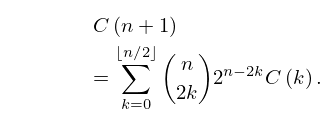
14: 26.5 Lattice Paths: Catalan Numbers

… ►

26.5.1 $$C\left(n\right)=\frac{1}{n+1}\left(\genfrac{}{}{0.0pt}{}{2n}{n}\right)=\frac{1}{2n+1}\left(\genfrac{}{}{0.0pt}{}{2n+1}{n}\right)=\left(\genfrac{}{}{0.0pt}{}{2n}{n}\right)-\left(\genfrac{}{}{0.0pt}{}{2n}{n-1}\right)=\left(\genfrac{}{}{0.0pt}{}{2n-1}{n}\right)-\left(\genfrac{}{}{0.0pt}{}{2n-1}{n+1}\right).$$

ⓘ

Defines:

$C\left(n\right)$: Catalan number

Symbols:

$\left(\genfrac{}{}{0.0pt}{}{m}{n}\right)$: binomial coefficient and $n$: nonnegative integer

Referenced by:

§26.5(iv)

Permalink:

http://dlmf.nist.gov/26.5.E1

Encodings:

pMML, png, TeX

See also:

Annotations for §26.5(i), §26.5 and Ch.26

… ►

Table 26.5.1: Catalan numbers.

► ►►►

$n$	$C\left(n\right)$	$n$	$C\left(n\right)$	$n$	$C\left(n\right)$
…
6	132	13	7 42900	20	65641 20420

►

… ►

26.5.5 $$C\left(n+1\right)=\sum _{k=0}^{\lfloor n/2\rfloor }\left(\genfrac{}{}{0.0pt}{}{n}{2k}\right)2^{n-2k}C\left(k\right).$$

ⓘ

Symbols:

$C\left(n\right)$: Catalan number, $\left(\genfrac{}{}{0.0pt}{}{m}{n}\right)$: binomial coefficient, $\lfloor x\rfloor$: floor of $x$ , $k$: nonnegative integer and $n$: nonnegative integer

Permalink:

http://dlmf.nist.gov/26.5.E5

Encodings:

pMML, png, TeX

See also:

Annotations for §26.5(iii), §26.5 and Ch.26

…

15: Bibliography N

… ►

Tables of Lagrangian Interpolation Coefficients. Columbia University Press, New York.

ⓘ

Notes:

Technical Director: Arnold N. Lowan

External Links:

MathReview (W. Feller), ZentralBlatt

Referenced by:

§3.3(ii).

Encodings:

BibTeX

… ►

On an integral transform involving a class of Mathieu functions. SIAM J. Math. Anal. 20 (6), pp. 1500–1513.

ⓘ

External Links:

ISSN 0036-1410, Document, MathReview (K. C. Gupta), ZentralBlatt

Referenced by:

§28.26(ii).

Encodings:

BibTeX

… ►

Tables Relating to Mathieu Functions: Characteristic Values, Coefficients, and Joining Factors. 2nd edition, National Bureau of Standards Applied Mathematics Series, U.S. Government Printing Office, Washington, D.C..

ⓘ

External Links:

MathReview, ZentralBlatt

Referenced by:

§28.1, §28.26(i), 6th item, Notations S, Notations S.

Encodings:

BibTeX

… ►

Reduction and evaluation of elliptic integrals. Math. Comp. 20 (94), pp. 223–231.

ⓘ

External Links:

FullText, MathReview (I. A. Stegun), ZentralBlatt

Referenced by:

§19.37(iv).

Encodings:

BibTeX

… ►

A table of integrals of the error functions. J. Res. Nat. Bur. Standards Sect B. 73B, pp. 1–20.

ⓘ

Notes:

See for additions and corrections same journal, Sect. B 75, 149–163 (1975)

External Links:

MathReview, ZentralBlatt

Referenced by:

§7.14(iii), §7.21, §7.7(iii).

Encodings:

BibTeX

…

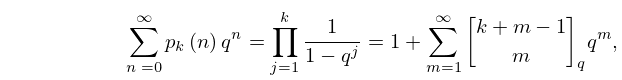
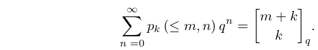
16: 26.9 Integer Partitions: Restricted Number and Part Size

… ►

26.9.4 $${\left[\genfrac{}{}{0.0pt}{}{m}{n}\right]}_q=\prod _{j=1}^n\frac{1-q^{m-n+j}}{1-q^j},$$ $n\ge 0$,

ⓘ

Symbols:

${\left[\genfrac{}{}{0.0pt}{}{n}{m}\right]}_q$: $q$-binomial coefficient (or Gaussian polynomial), $j$: nonnegative integer, $m$: nonnegative integer, $n$: nonnegative integer and $q$: parameter

Permalink:

http://dlmf.nist.gov/26.9.E4

Encodings:

pMML, png, TeX

See also:

Annotations for §26.9(ii), §26.9 and Ch.26

►is the Gaussian polynomial (or $q$-binomial coefficient); see also §§17.2(i)–17.2(ii). … ►

26.9.5 $$\sum _{n=0}^{\mathrm{\infty }}{p}_k\left(n\right)q^n=\prod _{j=1}^k\frac{1}{1-q^j}=1+\sum _{m=1}^{\mathrm{\infty }}{\left[\genfrac{}{}{0.0pt}{}{k+m-1}{m}\right]}_q{q}^m,$$

ⓘ

Symbols:

$p_k\left(n\right)$: total number of partitions of $n$ into at most $k$ parts, ${\left[\genfrac{}{}{0.0pt}{}{n}{m}\right]}_q$: $q$-binomial coefficient (or Gaussian polynomial), $j$: nonnegative integer, $k$: nonnegative integer, $m$: nonnegative integer, $n$: nonnegative integer and $q$: parameter

Permalink:

http://dlmf.nist.gov/26.9.E5

Encodings:

pMML, png, TeX

See also:

Annotations for §26.9(ii), §26.9 and Ch.26

►

26.9.6 $$\sum _{n=0}^{\mathrm{\infty }}{p}_k(\le m,n)q^n={\left[\genfrac{}{}{0.0pt}{}{m+k}{k}\right]}_q.$$

ⓘ

Symbols:

${\left[\genfrac{}{}{0.0pt}{}{n}{m}\right]}_q$: $q$-binomial coefficient (or Gaussian polynomial), $p_k(\le m,n)$: number of partitions of $n$ into at most $k$ parts, each less than or equal to $m$ , $k$: nonnegative integer, $m$: nonnegative integer, $n$: nonnegative integer and $q$: parameter

Permalink:

http://dlmf.nist.gov/26.9.E6

Encodings:

pMML, png, TeX

See also:

Annotations for §26.9(ii), §26.9 and Ch.26

… ►

26.9.7 $$\sum _{m,n=0}^{\mathrm{\infty }}{p}_k(\le m,n)x^k{q}^n=1+\sum _{k=1}^{\mathrm{\infty }}{\left[\genfrac{}{}{0.0pt}{}{m+k}{k}\right]}_q{x}^k=\prod _{j=0}^m\frac{1}{1-x{q}^j}.$$

ⓘ

Symbols:

${\left[\genfrac{}{}{0.0pt}{}{n}{m}\right]}_q$: $q$-binomial coefficient (or Gaussian polynomial), $p_k(\le m,n)$: number of partitions of $n$ into at most $k$ parts, each less than or equal to $m$ , $x$: real variable, $j$: nonnegative integer, $k$: nonnegative integer, $m$: nonnegative integer, $n$: nonnegative integer and $q$: parameter

Permalink:

http://dlmf.nist.gov/26.9.E7

Encodings:

pMML, png, TeX

See also:

Annotations for §26.9(ii), §26.9 and Ch.26

…

17: 8.26 Tables

… ►

Khamis (1965) tabulates $P(a,x)$ for $a=0.05(.05)10(.1)20(.25)70$, $0.0001\le x\le 250$ to 10D.

… ►

Abramowitz and Stegun (1964, pp. 245–248) tabulates $E_n\left(x\right)$ for $n=2,3,4,10,20$, $x=0(.01)2$ to 7D; also $(x+n){\mathrm{e}}^x{E}_n\left(x\right)$ for $n=2,3,4,10,20$, $x^{-1}=0(.01)0.1(.05)0.5$ to 6S.

… ►

Pagurova (1961) tabulates $E_n\left(x\right)$ for $n=0(1)20$, $x=0(.01)2(.1)10$ to 4-9S; ${\mathrm{e}}^x{E}_n\left(x\right)$ for $n=2(1)10$, $x=10(.1)20$ to 7D; ${\mathrm{e}}^x{E}_p\left(x\right)$ for $p=0(.1)1$, $x=0.01(.01)7(.05)12(.1)20$ to 7S or 7D.

… ►

Zhang and Jin (1996, Table 19.1) tabulates $E_n\left(x\right)$ for $n=1,2,3,5,10,15,20$, $x=0(.1)1,1.5,2,3,5,10,20,30,50,100$ to 7D or 8S.

18: 23 Weierstrass Elliptic and Modular
Functions

…

19: 5.11 Asymptotic Expansions

… ►where … ►

5.11.5 $$g_k=\sqrt{2}{\left(\frac{1}{2}\right)}_k{a}_{2k},$$

ⓘ

Symbols:

${\left(a\right)}_n$: Pochhammer’s symbol (or shifted factorial), $k$: nonnegative integer, $g_k$: coefficients and $a_k$: coefficient

Referenced by:

§5.11(i)

Permalink:

http://dlmf.nist.gov/5.11.E5

Encodings:

pMML, png, TeX

See also:

Annotations for §5.11(i), §5.11 and Ch.5

►where $a_0=\frac{1}{2}\sqrt{2}$ and …Wrench (1968) gives exact values of $g_k$ up to $g_{20}$. … ►

5.11.17 $$G_k(a,b)=\left(\genfrac{}{}{0.0pt}{}{a-b}{k}\right)B_k^{(a-b+1)}\left(a\right),$$

ⓘ

Defines:

$G_k(a,b)$: coefficients (locally)

Symbols:

$\left(\genfrac{}{}{0.0pt}{}{m}{n}\right)$: binomial coefficient, $B_n^{(\mathrm{\ell })}\left(x\right)$: generalized Bernoulli polynomials, $k$: nonnegative integer, $a$: real or complex variable and $b$: real or complex variable

Permalink:

http://dlmf.nist.gov/5.11.E17

Encodings:

pMML, png, TeX

See also:

Annotations for §5.11(iii), §5.11 and Ch.5

…

20: 12.11 Zeros

… ►The first two coefficients are given by ►

12.11.5 $$p_0(\zeta )=t(\zeta ),$$

ⓘ

Symbols:

$\zeta$: change of variable and $p_n(\zeta )$: coefficients

Permalink:

http://dlmf.nist.gov/12.11.E5

Encodings:

pMML, png, TeX

See also:

Annotations for §12.11(iii), §12.11 and Ch.12

… ►

12.11.6 $$p_1(\zeta )=\frac{t^3-6t}{24{(t^2-1)}^2}+\frac{5}{48{((t^2-1){\zeta }^3)}^{\frac{1}{2}}}.$$

ⓘ

Symbols:

$\zeta$: change of variable and $p_n(\zeta )$: coefficients

Permalink:

http://dlmf.nist.gov/12.11.E6

Encodings:

pMML, png, TeX

See also:

Annotations for §12.11(iii), §12.11 and Ch.12

… ►

12.11.9 $$u_{a,1}\sim 2^{\frac{1}{2}}\mu \left(1-\mathrm{1.85575\hspace{0.33em}708}{\mu }^{-4/3}-\mathrm{0.34438\hspace{0.33em}34}{\mu }^{-8/3}-\mathrm{0.16871\hspace{0.33em}5}{\mu }^{-4}-0.11414{\mu }^{-16/3}-0.0808{\mu }^{-20/3}-\mathrm{\cdots }\right),$$

ⓘ

Symbols:

$\sim$: Poincaré asymptotic expansion, $a$: real or complex parameter and $u_{a,s}$: zeros

Referenced by:

§12.11(iii)

Permalink:

http://dlmf.nist.gov/12.11.E9

Encodings:

pMML, png, TeX

See also:

Annotations for §12.11(iii), §12.11 and Ch.12

►where the numerical coefficients have been rounded off. …