isolated%20essential

♦ 11—20 of 118 matching pages ♦

(0.001 seconds)

11—20 of 118 matching pages

11: 8.26 Tables

… ►

•

Khamis (1965) tabulates $P\left(a,x\right)$ for $a=0.05(.05)10(.1)20(.25)70$ , $0.0001\leq x\leq 250$ to 10D.

… ►

•

Abramowitz and Stegun (1964, pp. 245–248) tabulates $E_{n}\left(x\right)$ for $n=2,3,4,10,20$ , $x=0(.01)2$ to 7D; also $(x+n)e^{x}E_{n}\left(x\right)$ for $n=2,3,4,10,20$ , $x^{-1}=0(.01)0.1(.05)0.5$ to 6S.

… ►

•

Pagurova (1961) tabulates $E_{n}\left(x\right)$ for $n=0(1)20$ , $x=0(.01)2(.1)10$ to 4-9S; $e^{x}E_{n}\left(x\right)$ for $n=2(1)10$ , $x=10(.1)20$ to 7D; $e^{x}E_{p}\left(x\right)$ for $p=0(.1)1$ , $x=0.01(.01)7(.05)12(.1)20$ to 7S or 7D.

… ►

•

Zhang and Jin (1996, Table 19.1) tabulates $E_{n}\left(x\right)$ for $n=1,2,3,5,10,15,20$ , $x=0(.1)1,1.5,2,3,5,10,20,30,50,100$ to 7D or 8S.

12: 23 Weierstrass Elliptic and Modular
Functions

…

13: 18.39 Applications in the Physical Sciences

… ►Derivations of (18.39.42) appear in Bethe and Salpeter (1957, pp. 12–20), and Pauling and Wilson (1985, Chapter V and Appendix VII), where the derivations are based on (18.39.36), and is also the notation of Piela (2014, §4.7), typifying the common use of the associated Coulomb–Laguerre polynomials in theoretical quantum chemistry. … ►

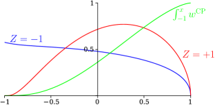
See accompanying text — Figure 18.39.2: Coulomb–Pollaczek weight functions, $x\in[-1,1]$ , (18.39.50) for $s=10$ , $l=0$ , and $Z=\pm 1$ . For $Z=+1$ the weight function, red curve, has an essential singularity at $x=-1$ , as all derivatives vanish as $x\to-1{+}$ ; the green curve is $\int_{-1}^{x}w^{\mathrm{CP}}(y)\,\mathrm{d}y$ , to be compared with its *histogram approximation* in §18.40(ii). For $Z=-1$ the weight function, blue curve, is non-zero at $x=-1$ , but this point is also an essential singularity as the discrete parts of the weight function of (18.39.51) accumulate as $k\to\infty$ , $x_{k}\to-1{-}$ . Magnify

… ►The Schrödinger operator essential singularity, seen in the accumulation of discrete eigenvalues for the attractive Coulomb problem, is mirrored in the accumulation of jumps in the discrete Pollaczek–Stieltjes measure as

x\to-1{-}

. …

14: 19.36 Methods of Computation

… ►

19.36.2

1-\tfrac{3}{14}E_{2}+\tfrac{1}{6}E_{3}+\tfrac{9}{88}E_{2}^{2}-\tfrac{3}{22}E_{% 4}-\tfrac{9}{52}E_{2}E_{3}+\tfrac{3}{26}E_{5}-\tfrac{1}{16}E_{2}^{3}+\tfrac{3}% {40}E_{3}^{2}+\tfrac{3}{20}E_{2}E_{4}+\tfrac{45}{272}E_{2}^{2}E_{3}-\tfrac{9}{% 68}(E_{3}E_{4}+E_{2}E_{5}).

ⓘ

Symbols:: $E_{s}(\mathbf{z})$ : symmetric function
Referenced by:: §19.19
Permalink:: http://dlmf.nist.gov/19.36.E2
Encodings:: pMML, png, TeX
See also:: Annotations for §19.36(i), §19.36 and Ch.19

… ►All cases of

R_{F}

R_{C}

R_{J}

, and

R_{D}

are computed by essentially the same procedure (after transforming Cauchy principal values by means of (19.20.14) and (19.2.20)). … ►For computation of Legendre’s integral of the third kind, see Abramowitz and Stegun (1964, §§17.7 and 17.8, Examples 15, 17, 19, and 20). …

15: Notices

… ►The DLMF wishes to provide users of special functions with essential reference information related to the use and application of special functions in research, development, and education. …

16: 36 Integrals with Coalescing Saddles

…

17: Gergő Nemes

… ►As of September 20, 2021, Nemes performed a complete analysis and acted as main consultant for the update of the source citation and proof metadata for every formula in Chapter 25 Zeta and Related Functions. …

18: Wolter Groenevelt

… ►As of September 20, 2022, Groenevelt performed a complete analysis and acted as main consultant for the update of the source citation and proof metadata for every formula in Chapter 18 Orthogonal Polynomials. …

19: 33.24 Tables

… ►

•

Abramowitz and Stegun (1964, Chapter 14) tabulates $F_{0}\left(\eta,\rho\right)$ , $G_{0}\left(\eta,\rho\right)$ , $F_{0}'\left(\eta,\rho\right)$ , and $G_{0}'\left(\eta,\rho\right)$ for $\eta=0.5(.5)20$ and $\rho=1(1)20$ , 5S; $C_{0}\left(\eta\right)$ for $\eta=0(.05)3$ , 6S.

…

20: 27.15 Chinese Remainder Theorem

… ►Their product

m

has 20 digits, twice the number of digits in the data. …These numbers, in turn, are combined by the Chinese remainder theorem to obtain the final result

\pmod{m}

, which is correct to 20 digits. …