functions f(?,?;r),h(?,?;r)

SearchAdvancedHelp

(0.007 seconds)

1—10 of 84 matching pages

1: 33.15 Graphics

… ►

§33.15(i) Line Graphs of the Coulomb Functions $f(ϵ,\mathrm{\ell };r)$ and $h(ϵ,\mathrm{\ell };r)$

… ►

§33.15(ii) Surfaces of the Coulomb Functions $f(ϵ,\mathrm{\ell };r)$, $h(ϵ,\mathrm{\ell };r)$, $s(ϵ,\mathrm{\ell };r)$, and $c(ϵ,\mathrm{\ell };r)$

…

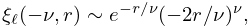
2: 33.18 Limiting Forms for Large $\mathrm{\ell }$

§33.18 Limiting Forms for Large $\mathrm{\ell }$

►As $\mathrm{\ell }\to \mathrm{\infty }$ with $ϵ$ and $r$ ($\ne 0$) fixed, ►

$f(ϵ,\mathrm{\ell };r)\sim {\displaystyle \frac{{(2r)}^{\mathrm{\ell }+1}}{(2\mathrm{\ell }+1)!}},$

►

$h(ϵ,\mathrm{\ell };r)\sim {\displaystyle \frac{(2\mathrm{\ell })!}{\pi {(2r)}^{\mathrm{\ell }}}}.$

3: 33.14 Definitions and Basic Properties

… ►

§33.14(ii) Regular Solution $f(ϵ,\mathrm{\ell };r)$

… ►

§33.14(iii) Irregular Solution $h(ϵ,\mathrm{\ell };r)$

…

4: 33.1 Special Notation

… ►The main functions treated in this chapter are first the Coulomb radial functions $F_{\mathrm{\ell }}(\eta ,\rho )$, $G_{\mathrm{\ell }}(\eta ,\rho )$, $H_{\mathrm{\ell }}^{\pm }(\eta ,\rho )$ (Sommerfeld (1928)), which are used in the case of repulsive Coulomb interactions, and secondly the functions $f(ϵ,\mathrm{\ell };r)$, $h(ϵ,\mathrm{\ell };r)$, $s(ϵ,\mathrm{\ell };r)$, $c(ϵ,\mathrm{\ell };r)$ (Seaton (1982, 2002a)), which are used in the case of attractive Coulomb interactions. …

5: 33.20 Expansions for Small $|ϵ|$

… ►

§33.20(i) Case $ϵ=0$

… ►where … ►where $A(ϵ,\mathrm{\ell })$ is given by (33.14.11), (33.14.12), and … ►

§33.20(iv) Uniform Asymptotic Expansions

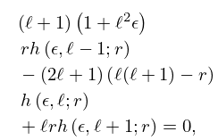
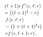
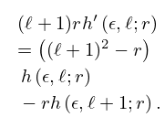
►For a comprehensive collection of asymptotic expansions that cover $f(ϵ,\mathrm{\ell };r)$ and $h(ϵ,\mathrm{\ell };r)$ as $ϵ\to 0\pm$ and are uniform in $r$, including unbounded values, see Curtis (1964a, §7). …

6: 33.17 Recurrence Relations and Derivatives

§33.17 Recurrence Relations and Derivatives

►

33.17.1 $$(\mathrm{\ell }+1)rf(ϵ,\mathrm{\ell }-1;r)-(2\mathrm{\ell }+1)\left(\mathrm{\ell }(\mathrm{\ell }+1)-r\right)f(ϵ,\mathrm{\ell };r)+\mathrm{\ell }\left(1+{(\mathrm{\ell }+1)}^2ϵ\right)rf(ϵ,\mathrm{\ell }+1;r)=0,$$

ⓘ

Symbols:

$f(ϵ,\mathrm{\ell };r)$: regular Coulomb function, $\mathrm{\ell }$: nonnegative integer, $r$: real variable and $ϵ$: real parameter

Permalink:

http://dlmf.nist.gov/33.17.E1

Encodings:

pMML, png, TeX

See also:

Annotations for §33.17 and Ch.33

►

33.17.2 $$(\mathrm{\ell }+1)\left(1+{\mathrm{\ell }}^2ϵ\right)rh(ϵ,\mathrm{\ell }-1;r)-(2\mathrm{\ell }+1)\left(\mathrm{\ell }(\mathrm{\ell }+1)-r\right)h(ϵ,\mathrm{\ell };r)+\mathrm{\ell }rh(ϵ,\mathrm{\ell }+1;r)=0,$$

ⓘ

Symbols:

$h(ϵ,\mathrm{\ell };r)$: irregular Coulomb function, $\mathrm{\ell }$: nonnegative integer, $r$: real variable and $ϵ$: real parameter

Permalink:

http://dlmf.nist.gov/33.17.E2

Encodings:

pMML, png, TeX

See also:

Annotations for §33.17 and Ch.33

►

33.17.3 $$(\mathrm{\ell }+1)r{f}^{\prime }(ϵ,\mathrm{\ell };r)=\left({(\mathrm{\ell }+1)}^2-r\right)f(ϵ,\mathrm{\ell };r)-\left(1+{(\mathrm{\ell }+1)}^2ϵ\right)rf(ϵ,\mathrm{\ell }+1;r),$$

ⓘ

Symbols:

$f(ϵ,\mathrm{\ell };r)$: regular Coulomb function, $\mathrm{\ell }$: nonnegative integer, $r$: real variable and $ϵ$: real parameter

Permalink:

http://dlmf.nist.gov/33.17.E3

Encodings:

pMML, png, TeX

See also:

Annotations for §33.17 and Ch.33

►

33.17.4 $$(\mathrm{\ell }+1)r{h}^{\prime }(ϵ,\mathrm{\ell };r)=\left({(\mathrm{\ell }+1)}^2-r\right)h(ϵ,\mathrm{\ell };r)-rh(ϵ,\mathrm{\ell }+1;r).$$

ⓘ

Symbols:

$h(ϵ,\mathrm{\ell };r)$: irregular Coulomb function, $\mathrm{\ell }$: nonnegative integer, $r$: real variable and $ϵ$: real parameter

Permalink:

http://dlmf.nist.gov/33.17.E4

Encodings:

pMML, png, TeX

See also:

Annotations for §33.17 and Ch.33

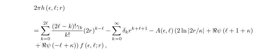
7: 33.19 Power-Series Expansions in $r$

… ►

33.19.3 $$2\pi h(ϵ,\mathrm{\ell };r)=\sum _{k=0}^{2\mathrm{\ell }}\frac{(2\mathrm{\ell }-k)!{\gamma }_k}{k!}{(2r)}^{k-\mathrm{\ell }}-\sum _{k=0}^{\mathrm{\infty }}{\delta }_k{r}^{k+\mathrm{\ell }+1}-A(ϵ,\mathrm{\ell })\left(2\ln |2r/\kappa |+\mathrm{\Re }\psi \left(\mathrm{\ell }+1+\kappa \right)+\mathrm{\Re }\psi \left(-\mathrm{\ell }+\kappa \right)\right)f(ϵ,\mathrm{\ell };r),$$ $r\ne 0$.

ⓘ

Symbols:

$f(ϵ,\mathrm{\ell };r)$: regular Coulomb function, $h(ϵ,\mathrm{\ell };r)$: irregular Coulomb function, $\pi$: the ratio of the circumference of a circle to its diameter, $\psi \left(z\right)$: psi (or digamma) function, $!$: factorial (as in $n!$), $\ln z$: principal branch of logarithm function, $\mathrm{\Re }$: real part, $k$: nonnegative integer, $\mathrm{\ell }$: nonnegative integer, $r$: real variable, $ϵ$: real parameter, $\kappa$: quantity, $A(ϵ,\mathrm{\ell })$: function, ${\gamma }_k$: term and ${\delta }_k$: term

Referenced by:

§33.19

Permalink:

http://dlmf.nist.gov/33.19.E3

Encodings:

pMML, png, TeX

See also:

Annotations for §33.19 and Ch.33

…

8: 24.17 Mathematical Applications

… ►

24.17.1 $$\sum _{j=a}^{n-1}{(-1)}^{j}f(j+h)=\frac{1}{2}\sum _{k=0}^{m-1}\frac{E_k\left(h\right)}{k!}\left({(-1)}^{n-1}{f}^{(k)}(n)+{(-1)}^a{f}^{(k)}(a)\right)+R_m(n),$$

ⓘ

Symbols:

$E_n\left(x\right)$: Euler polynomials, $!$: factorial (as in $n!$), $j$: integer, $k$: integer, $m$: integer, $h$: parameter, $a$: integer, $n$: integer, $f^{(m)}(x)$: integrable function and $R_m(n)$: remainder

Permalink:

http://dlmf.nist.gov/24.17.E1

Encodings:

pMML, png, TeX

See also:

Annotations for §24.17(i), §24.17(i), §24.17 and Ch.24

… ►

24.17.2 $$R_m(n)=\frac{1}{2(m-1)!}{\int }_a^n{f}^{(m)}(x){\tilde{E}}_{m-1}\left(h-x\right)dx.$$

ⓘ

Symbols:

$dx$: differential of $x$ , $!$: factorial (as in $n!$), $\int$: integral, ${\tilde{E}}_n\left(x\right)$: periodic Euler functions, $m$: integer, $x$: real or complex, $h$: parameter, $a$: integer, $n$: integer, $f^{(m)}(x)$: integrable function and $R_m(n)$: remainder

Permalink:

http://dlmf.nist.gov/24.17.E2

Encodings:

pMML, png, TeX

See also:

Annotations for §24.17(i), §24.17(i), §24.17 and Ch.24

…

9: 33.21 Asymptotic Approximations for Large $|r|$

… ►

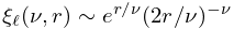
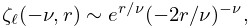
§33.21(i) Limiting Forms

►We indicate here how to obtain the limiting forms of $f(ϵ,\mathrm{\ell };r)$, $h(ϵ,\mathrm{\ell };r)$, $s(ϵ,\mathrm{\ell };r)$, and $c(ϵ,\mathrm{\ell };r)$ as $r\to \pm \mathrm{\infty }$, with $ϵ$ and $\mathrm{\ell }$ fixed, in the following cases: … ►

When $r\to \pm \mathrm{\infty }$ with , Equations (33.16.10)–(33.16.13) are combined with

33.21.1

${\zeta }_{\mathrm{\ell }}(\nu ,r)\sim {\mathrm{e}}^{-r/\nu }{(2r/\nu )}^{\nu },$

${\xi }_{\mathrm{\ell }}(\nu ,r)\sim {\mathrm{e}}^{r/\nu }{(2r/\nu )}^{-\nu }$ , $r\to \mathrm{\infty }$,

ⓘ

Symbols:

$\sim$: asymptotic equality, $\mathrm{e}$: base of natural logarithm, $\mathrm{\ell }$: nonnegative integer, $r$: real variable, $\nu$: parameter, ${\zeta }_{\mathrm{\ell }}(\nu ,r)$: function and ${\xi }_{\mathrm{\ell }}(\nu ,r)$: function

Permalink:

http://dlmf.nist.gov/33.21.E1

Encodings:

pMML, pMML, png, png, TeX, TeX

See also:

Annotations for §33.21(i), §33.21 and Ch.33

33.21.2

${\zeta }_{\mathrm{\ell }}(-\nu ,r)\sim {\mathrm{e}}^{r/\nu }{(-2r/\nu )}^{-\nu },$

${\xi }_{\mathrm{\ell }}(-\nu ,r)\sim {\mathrm{e}}^{-r/\nu }{(-2r/\nu )}^{\nu },$ $r\to -\mathrm{\infty }$.

ⓘ

Symbols:

$\sim$: asymptotic equality, $\mathrm{e}$: base of natural logarithm, $\mathrm{\ell }$: nonnegative integer, $r$: real variable, $\nu$: parameter, ${\zeta }_{\mathrm{\ell }}(\nu ,r)$: function and ${\xi }_{\mathrm{\ell }}(\nu ,r)$: function

Permalink:

http://dlmf.nist.gov/33.21.E2

Encodings:

pMML, pMML, png, png, TeX, TeX

See also:

Annotations for §33.21(i), §33.21 and Ch.33

Corresponding approximations for $s(ϵ,\mathrm{\ell };r)$ and $c(ϵ,\mathrm{\ell };r)$ as $r\to \mathrm{\infty }$ can be obtained via (33.16.17), and as $r\to -\mathrm{\infty }$ via (33.16.18).

… ►

§33.21(ii) Asymptotic Expansions

►For asymptotic expansions of $f(ϵ,\mathrm{\ell };r)$ and $h(ϵ,\mathrm{\ell };r)$ as $r\to \pm \mathrm{\infty }$ with $ϵ$ and $\mathrm{\ell }$ fixed, see Curtis (1964a, §6).

10: How to Cite

… ►

NIST Digital Library of Mathematical Functions. https://dlmf.nist.gov/, Release 1.2.2 of 2024-09-15. F. W. J. Olver, A. B. Olde Daalhuis, D. W. Lozier, B. I. Schneider, R. F. Boisvert, C. W. Clark, B. R. Miller, B. V. Saunders, H. S. Cohl, and M. A. McClain, eds.

…