central%20in%20imaginary%20direction
(0.003 seconds)
11—20 of 950 matching pages
11: 23 Weierstrass Elliptic and Modular
Functions
…
12: 36 Integrals with Coalescing Saddles
…
13: Peter L. Walker
…
► 1942 in Dorchester, U.
…He began his academic career in 1964 at the University of Lancaster, U.
…
►Walker’s books are An Introduction to Complex Analysis, published by Hilger in 1974, The Theory of Fourier Series and Integrals, published by Wiley in 1986, Elliptic Functions. A Constructive Approach, published by Wiley in 1996, and Examples and Theorems in Analysis, published by Springer in 2004.
…
►Walker is now retired and living in Cheltenham, UK.
…
►
…
14: William P. Reinhardt
…
►He currently resides in Santa Fe, NM.
►Reinhardt is a theoretical chemist and atomic physicist, who has always been interested in orthogonal polynomials and in the analyticity properties of the functions of mathematical physics.
…
►This is closely connected with his interests in classical dynamical “chaos,” an area where he coauthored a book, Chaos in atomic physics with Reinhold Blümel.
…
►
…
►In November 2015, Reinhardt was named Senior Associate Editor of the DLMF and Associate Editor for Chapters 20, 22, and 23.
15: 27.15 Chinese Remainder Theorem
…
►This theorem is employed to increase efficiency in calculating with large numbers by making use of smaller numbers in most of the calculation.
…Their product has 20 digits, twice the number of digits in the data.
By the Chinese remainder theorem each integer in the data can be uniquely represented by its residues (mod ), (mod ), (mod ), and (mod ), respectively.
…These numbers, in turn, are combined by the Chinese remainder theorem to obtain the final result , which is correct to 20 digits.
…
►Details of a machine program describing the method together with typical numerical results can be found in Newman (1967).
…
16: 18.20 Hahn Class: Explicit Representations
…
►For comments on the use of the forward-difference operator , the backward-difference operator , and the central-difference operator , see §18.2(ii).
…
►In (18.20.1) and are as in Table 18.19.1.
…For the Krawtchouk, Meixner, and Charlier polynomials, and are as in Table 18.20.1.
…
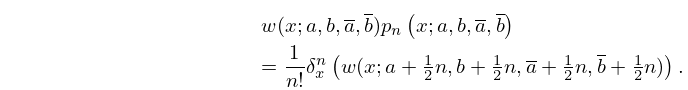
►
18.20.3
…
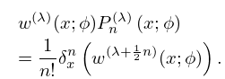
►
18.20.4
…
17: Bibliography C
…
►
Algorithm AS 310. Computing the non-central beta distribution function.
Appl. Statist. 46 (1), pp. 146–156.
…
►
Asymptotic estimates for generalized Stirling numbers.
Analysis (Munich) 20 (1), pp. 1–13.
…
►
Validated computation of certain hypergeometric functions.
ACM Trans. Math. Software 38 (2), pp. Art. 11, 20.
…
►
Some non-central distribution problems in multivariate analysis.
Ann. Math. Statist. 34 (4), pp. 1270–1285.
…
►
Coulomb effects in the Klein-Gordon equation for pions.
Phys. Rev. C 20 (2), pp. 696–704.
…
18: 18.39 Applications in the Physical Sciences
§18.39 Applications in the Physical Sciences
… ►The spectrum is entirely discrete as in §1.18(v). … ►In what follows the radial and spherical radial eigenfunctions corresponding to (18.39.27) are found in four different notations, with identical eigenvalues, all of which appear in the current and past mathematical and theoretical physics and chemistry literatures, regarding this central problem. … ►Derivations of (18.39.42) appear in Bethe and Salpeter (1957, pp. 12–20), and Pauling and Wilson (1985, Chapter V and Appendix VII), where the derivations are based on (18.39.36), and is also the notation of Piela (2014, §4.7), typifying the common use of the associated Coulomb–Laguerre polynomials in theoretical quantum chemistry. … ►§18.39(iii) Non Classical Weight Functions of Utility in DVR Method in the Physical Sciences
…19: 18.22 Hahn Class: Recurrence Relations and Differences
…
►
§18.22(i) Recurrence Relations in
… ►These polynomials satisfy (18.22.2) with , , and as in Table 18.22.1. … ►§18.22(ii) Difference Equations in
… ►For , , and in (18.22.12) see Table 18.22.2. … ►
18.22.27
…
20: 10.75 Tables
…
►
•
…
►
•
…
►
•
►
•
…
►
•
…
Achenbach (1986) tabulates , , , , , 20D or 18–20S.
Bickley et al. (1952) tabulates or , or , , (.01 or .1) 10(.1) 20, 8S; , , , or , 10S.
Kerimov and Skorokhodov (1984b) tabulates all zeros of the principal values of and , for , 9S.
Kerimov and Skorokhodov (1984c) tabulates all zeros of and in the sector for , 9S.
