Nörlund polynomials

♦ 1—10 of 13 matching pages ♦

(0.001 seconds)

1—10 of 13 matching pages

1: 24.16 Generalizations

… ►

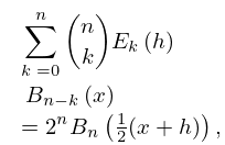
Nörlund Polynomials

…

2: 24.2 Definitions and Generating Functions

… ►

§24.2(i) Bernoulli Numbers and Polynomials

… ►

§24.2(ii) Euler Numbers and Polynomials

… ►

(-1)^{n}E_{2n}>0

… ►

Table 24.2.2: Bernoulli and Euler polynomials.

► ►►

$n$	$B_{n}\left(x\right)$	$E_{n}\left(x\right)$
…

► …

3: Bibliography C

… ►

L. Carlitz (1960) Note on Nörlund’s polynomial

B_{n}^{(z)}

. Proc. Amer. Math. Soc. 11 (3), pp. 452–455.

ⓘ

External Links:: FullText, MathReview (M. P. Drazin), ZentralBlatt
Referenced by:: §26.1, §26.1, Notations S, Notations S.
Encodings:: BibTeX

…

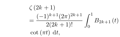
4: 24.13 Integrals

… ►

§24.13(i) Bernoulli Polynomials

… ►

24.13.3

\int_{x}^{x+(1/2)}B_{n}\left(t\right)\,\mathrm{d}t=\frac{E_{n}\left(2x\right)}% {2^{n+1}},

ⓘ

Symbols:: $B_{\NVar{n}}\left(\NVar{x}\right)$ : Bernoulli polynomials, $E_{\NVar{n}}\left(\NVar{x}\right)$ : Euler polynomials, $\,\mathrm{d}\NVar{x}$ : differential of $x$ , $\int$ : integral, $n$ : integer, $t$ : real or complex and $x$ : real or complex
Referenced by:: §24.13(i)
Permalink:: http://dlmf.nist.gov/24.13.E3
Encodings:: pMML, png, TeX
See also:: Annotations for §24.13(i), §24.13 and Ch.24

… ►For integrals of the form

\int_{0}^{x}B_{n}\left(t\right)B_{m}\left(t\right)\,\mathrm{d}t

and

\int_{0}^{x}B_{n}\left(t\right)B_{m}\left(t\right)B_{k}\left(t\right)\,\mathrm% {d}t

see Agoh and Dilcher (2011). ►

§24.13(ii) Euler Polynomials

… ►

§24.13(iii) Compendia

…

5: 24.1 Special Notation

… ►The notations

E_{n}

E_{n}\left(x\right)

, as defined in §24.2(ii), were used in Lucas (1891) and Nörlund (1924). …

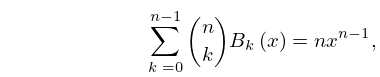
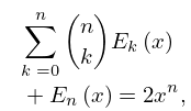
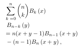
6: 24 Bernoulli and Euler Polynomials

Chapter 24 Bernoulli and Euler Polynomials

…

7: 24.4 Basic Properties

… ►

§24.4(i) Difference Equations

… ►

§24.4(ii) Symmetry

… ►Next, … ►

§24.4(vi) Special Values

… ►

§24.4(vii) Derivatives

…

8: 25.6 Integer Arguments

… ►

25.6.6

\zeta\left(2k+1\right)=\frac{(-1)^{k+1}(2\pi)^{2k+1}}{2(2k+1)!}\int_{0}^{1}B_{% 2k+1}\left(t\right)\cot\left(\pi t\right)\,\mathrm{d}t,

k=1,2,3,\dots

ⓘ

Symbols:: $B_{\NVar{n}}\left(\NVar{x}\right)$ : Bernoulli polynomials, $\zeta\left(\NVar{s}\right)$ : Riemann zeta function, $\pi$ : the ratio of the circumference of a circle to its diameter, $\cot\NVar{z}$ : cotangent function, $\,\mathrm{d}\NVar{x}$ : differential of $x$ , $!$ : factorial (as in $n!$ ), $\int$ : integral and $k$ : nonnegative integer
Source:: Nörlund (1924, (81*), p. 66); with $\nu=k$
A&S Ref:: 23.2.17
Permalink:: http://dlmf.nist.gov/25.6.E6
Encodings:: pMML, png, TeX
See also:: Annotations for §25.6(i), §25.6 and Ch.25

…

9: 24.5 Recurrence Relations

§24.5 Recurrence Relations

… ►

24.5.1

\sum_{k=0}^{n-1}{n\choose k}B_{k}\left(x\right)=nx^{n-1},

n=2,3,\dots

ⓘ

Symbols:: $B_{\NVar{n}}\left(\NVar{x}\right)$ : Bernoulli polynomials, $\genfrac{(}{)}{0.0pt}{}{\NVar{m}}{\NVar{n}}$ : binomial coefficient, $k$ : integer, $n$ : integer and $x$ : real or complex
Permalink:: http://dlmf.nist.gov/24.5.E1
Encodings:: pMML, png, TeX
See also:: Annotations for §24.5(i), §24.5 and Ch.24

►

24.5.2

\sum_{k=0}^{n}{n\choose k}E_{k}\left(x\right)+E_{n}\left(x\right)=2x^{n},

n=1,2,\dots

ⓘ

Symbols:: $E_{\NVar{n}}\left(\NVar{x}\right)$ : Euler polynomials, $\genfrac{(}{)}{0.0pt}{}{\NVar{m}}{\NVar{n}}$ : binomial coefficient, $k$ : integer, $n$ : integer and $x$ : real or complex
Permalink:: http://dlmf.nist.gov/24.5.E2
Encodings:: pMML, png, TeX
See also:: Annotations for §24.5(i), §24.5 and Ch.24

…

10: 24.14 Sums

§24.14 Sums

►

§24.14(i) Quadratic Recurrence Relations

►

24.14.1

\sum_{k=0}^{n}{n\choose k}B_{k}\left(x\right)B_{n-k}\left(y\right)=n(x+y-1)B_{% n-1}\left(x+y\right)-(n-1)B_{n}\left(x+y\right),

ⓘ

Symbols:: $B_{\NVar{n}}\left(\NVar{x}\right)$ : Bernoulli polynomials, $\genfrac{(}{)}{0.0pt}{}{\NVar{m}}{\NVar{n}}$ : binomial coefficient, $k$ : integer, $n$ : integer and $x$ : real or complex
Referenced by:: §24.14(i)
Permalink:: http://dlmf.nist.gov/24.14.E1
Encodings:: pMML, png, TeX
See also:: Annotations for §24.14(i), §24.14 and Ch.24

… ►

24.14.5

\sum_{k=0}^{n}{n\choose k}E_{k}\left(h\right)B_{n-k}\left(x\right)=2^{n}B_{n}% \left(\tfrac{1}{2}(x+h)\right),

ⓘ

Symbols:: $B_{\NVar{n}}\left(\NVar{x}\right)$ : Bernoulli polynomials, $E_{\NVar{n}}\left(\NVar{x}\right)$ : Euler polynomials, $\genfrac{(}{)}{0.0pt}{}{\NVar{m}}{\NVar{n}}$ : binomial coefficient, $k$ : integer, $n$ : integer and $x$ : real or complex
Permalink:: http://dlmf.nist.gov/24.14.E5
Encodings:: pMML, png, TeX
See also:: Annotations for §24.14(i), §24.14 and Ch.24

… ►For other sums involving Bernoulli and Euler numbers and polynomials see Hansen (1975, pp. 331–347) and Prudnikov et al. (1990, pp. 383–386).