Legendre

SearchAdvancedHelp

(0.001 seconds)

11—20 of 168 matching pages

11: 14.4 Graphics

… ►

§14.4(iii) Associated Legendre Functions: 2D Graphs

… ►

►►

Figure 14.4.24: ${𝑸}_0^{\mu }\left(x\right)$, $\mu =0,2,4,8$. Magnify

… ►

►►

Figure 14.4.28: ${𝑸}_1^{\mu }\left(x\right)$, $\mu =0,2,4,8$. Magnify

►

§14.4(iv) Associated Legendre Functions: 3D Surfaces

… ►

►

►

Figure 14.4.32: ${𝑸}_0^{\mu }\left(x\right)$, $0\le \mu \le 10$, . Magnify 3D Help

12: 14.2 Differential Equations

… ►

§14.2(i) Legendre’s Equation

… ►Standard solutions: ${𝖯}_{\nu }\left(\pm x\right)$, ${𝖰}_{\nu }\left(\pm x\right)$, ${𝖰}_{-\nu -1}\left(\pm x\right)$, $P_{\nu }\left(\pm x\right)$, $Q_{\nu }\left(\pm x\right)$, $Q_{-\nu -1}\left(\pm x\right)$. … ►

§14.2(ii) Associated Legendre Equation

… ►Ferrers functions and the associated Legendre functions are related to the Legendre functions by the equations ${𝖯}_{\nu }^0\left(x\right)={𝖯}_{\nu }\left(x\right)$, ${𝖰}_{\nu }^0\left(x\right)={𝖰}_{\nu }\left(x\right)$, $P_{\nu }^0\left(x\right)=P_{\nu }\left(x\right)$, $Q_{\nu }^0\left(x\right)=Q_{\nu }\left(x\right)$, ${𝑸}_{\nu }^0\left(x\right)={𝑸}_{\nu }\left(x\right)=Q_{\nu }\left(x\right)/\mathrm{\Gamma }\left(\nu +1\right)$. … ►

§14.2(iii) Numerically Satisfactory Solutions

…

13: 14.9 Connection Formulas

… ►

§14.9(i) Connections Between ${𝖯}_{\nu }^{\pm \mu }\left(x\right)$, ${𝖯}_{-\nu -1}^{\pm \mu }\left(x\right)$, ${𝖰}_{\nu }^{\pm \mu }\left(x\right)$, ${𝖰}_{-\nu -1}^{\mu }\left(x\right)$

… ►

${𝖯}_{-\nu -1}^{\mu }\left(x\right)={𝖯}_{\nu }^{\mu }\left(x\right),$

… ►

§14.9(ii) Connections Between ${𝖯}_{\nu }^{\pm \mu }\left(\pm x\right)$, ${𝖰}_{\nu }^{-\mu }\left(\pm x\right)$, ${𝖰}_{\nu }^{\mu }\left(x\right)$

… ►

§14.9(iii) Connections Between $P_{\nu }^{\pm \mu }\left(x\right)$, $P_{-\nu -1}^{\pm \mu }\left(x\right)$, ${𝑸}_{\nu }^{\pm \mu }\left(x\right)$, ${𝑸}_{-\nu -1}^{\mu }\left(x\right)$

… ►

§14.9(iv) Whipple’s Formula

…

14: 14.10 Recurrence Relations and Derivatives

§14.10 Recurrence Relations and Derivatives

… ► ${𝖰}_{\nu }^{\mu }\left(x\right)$ also satisfies (14.10.1)–(14.10.5). ►

14.10.6 $$P_{\nu }^{\mu +2}\left(x\right)+2(\mu +1)x{\left(x^2-1\right)}^{-1/2}{P}_{\nu }^{\mu +1}\left(x\right)-(\nu -\mu )(\nu +\mu +1)P_{\nu }^{\mu }\left(x\right)=0,$$

ⓘ

Symbols:

$P_{\nu }^{\mu }\left(z\right)$: associated Legendre function of the first kind, $x$: real variable, $\mu$: general order and $\nu$: general degree

Referenced by:

§14.10, §14.14

Permalink:

http://dlmf.nist.gov/14.10.E6

Encodings:

pMML, png, TeX

See also:

Annotations for §14.10 and Ch.14

… ► $Q_{\nu }^{\mu }\left(x\right)$ also satisfies (14.10.6) and (14.10.7). In addition, $P_{\nu }^{\mu }\left(x\right)$ and $Q_{\nu }^{\mu }\left(x\right)$ satisfy (14.10.3)–(14.10.5).

15: 14.22 Graphics

§14.22 Graphics

… ►

►

►

Figure 14.22.1: $P_{1/2}^0\left(x+\mathrm{i}y\right)$, $-5\le x\le 5$, $-5\le y\le 5$. … Magnify 3D Help

►

►

►

Figure 14.22.2: $P_{1/2}^{-1/2}\left(x+\mathrm{i}y\right)$, $-5\le x\le 5$, $-5\le y\le 5$. … Magnify 3D Help

… ►

►

►

Figure 14.22.4: ${𝑸}_0^0\left(x+\mathrm{i}y\right)$, $-5\le x\le 5$, $-5\le y\le 5$. … Magnify 3D Help

16: 14.28 Sums

§14.28 Sums

►

§14.28(i) Addition Theorem

… ►

14.28.1 $$P_{\nu }\left(z_1{z}_2-{\left(z_1^2-1\right)}^{1/2}{\left(z_2^2-1\right)}^{1/2}\cos \varphi \right)=P_{\nu }\left(z_1\right)P_{\nu }\left(z_2\right)+2\sum _{m=1}^{\mathrm{\infty }}{(-1)}^m\frac{\mathrm{\Gamma }\left(\nu -m+1\right)}{\mathrm{\Gamma }\left(\nu +m+1\right)}{P}_{\nu }^m\left(z_1\right)P_{\nu }^m(z_2)\cos \left(m\varphi \right),$$

ⓘ

Symbols:

$\mathrm{\Gamma }\left(z\right)$: gamma function, $P_{\nu }^{\mu }\left(z\right)$: associated Legendre function of the first kind, $\cos z$: cosine function, $P_{\nu }\left(z\right)=P_{\nu }^0\left(z\right)$: Legendre function of the first kind, $z$: complex variable, $m$: nonnegative integer and $\nu$: general degree

Permalink:

http://dlmf.nist.gov/14.28.E1

Encodings:

pMML, png, TeX

See also:

Annotations for §14.28(i), §14.28 and Ch.14

… ►

§14.28(ii) Heine’s Formula

►

14.28.2 $$\sum _{n=0}^{\mathrm{\infty }}(2n+1)Q_n\left(z_1\right)P_n\left(z_2\right)=\frac{1}{z_1-z_2},$$ $z_1\in {ℰ}_1$, $z_2\in {ℰ}_2$,

ⓘ

Symbols:

$\in$: element of, $P_{\nu }\left(z\right)=P_{\nu }^0\left(z\right)$: Legendre function of the first kind, $Q_{\nu }\left(z\right)=Q_{\nu }^0\left(z\right)$: Legendre function of the second kind, $z$: complex variable, $n$: nonnegative integer and ${ℰ}_1$, ${ℰ}_2$: ellipses

Permalink:

http://dlmf.nist.gov/14.28.E2

Encodings:

pMML, png, TeX

See also:

Annotations for §14.28(ii), §14.28 and Ch.14

…

17: 14.33 Tables

§14.33 Tables

►

Abramowitz and Stegun (1964, Chapter 8) tabulates ${𝖯}_n\left(x\right)$ for $n=0(1)3,9,10$, $x=0(.01)1$, 5–8D; ${𝖯}_n^{\prime }\left(x\right)$ for $n=1(1)4,9,10$, $x=0(.01)1$, 5–7D; ${𝖰}_n\left(x\right)$ and ${𝖰}_n^{\prime }\left(x\right)$ for $n=0(1)3,9,10$, $x=0(.01)1$, 6–8D; $P_n\left(x\right)$ and $P_n^{\prime }\left(x\right)$ for $n=0(1)5,9,10$, $x=1(.2)10$, 6S; $Q_n\left(x\right)$ and $Q_n^{\prime }\left(x\right)$ for $n=0(1)3,9,10$, $x=1(.2)10$, 6S. (Here primes denote derivatives with respect to $x$.)

►

Zhang and Jin (1996, Chapter 4) tabulates ${𝖯}_n\left(x\right)$ for $n=2(1)5,10$, $x=0(.1)1$, 7D; ${𝖯}_n\left(\cos \theta \right)$ for $n=1(1)4,10$, $\theta =0(5^{\circ }){90}^{\circ }$, 8D; ${𝖰}_n\left(x\right)$ for $n=0(1)2,10$, $x=0(.1)0.9$, 8S; ${𝖰}_n\left(\cos \theta \right)$ for $n=0(1)3,10$, $\theta =0(5^{\circ }){90}^{\circ }$, 8D; ${𝖯}_n^m\left(x\right)$ for $m=1(1)4$, $n-m=0(1)2$, $n=10$, $x=0,0.5$, 8S; ${𝖰}_n^m\left(x\right)$ for $m=1(1)4$, $n=0(1)2,10$, 8S; ${𝖯}_{\nu }^m\left(\cos \theta \right)$ for $m=0(1)3$, $\nu =0(.25)5$, $\theta =0({15}^{\circ }){90}^{\circ }$, 5D; $P_n\left(x\right)$ for $n=2(1)5,10$, $x=1(1)10$, 7S; $Q_n\left(x\right)$ for $n=0(1)2,10$, $x=2(1)10$, 8S. Corresponding values of the derivative of each function are also included, as are 6D values of the first 5 $\nu$-zeros of ${𝖯}_{\nu }^m\left(\cos \theta \right)$ and of its derivative for $m=0(1)4$, $\theta ={10}^{\circ },{30}^{\circ },{150}^{\circ }$.

… ►

Žurina and Karmazina (1964, 1965) tabulate the conical functions ${𝖯}_{-\frac{1}{2}+\mathrm{i}\tau }\left(x\right)$ for $\tau =0(.01)50$, $x=-0.9(.1)0.9$, 7S; $P_{-\frac{1}{2}+\mathrm{i}\tau }\left(x\right)$ for $\tau =0(.01)50$, $x=1.1(.1)2(.2)5(.5)10(10)60$, 7D. Auxiliary tables are included to facilitate computation for larger values of $\tau$ when .

►

Žurina and Karmazina (1963) tabulates the conical functions ${𝖯}_{-\frac{1}{2}+\mathrm{i}\tau }^1\left(x\right)$ for $\tau =0(.01)25$, $x=-0.9(.1)0.9$, 7S; $P_{-\frac{1}{2}+\mathrm{i}\tau }^1\left(x\right)$ for $\tau =0(.01)25$, $x=1.1(.1)2(.2)5(.5)10(10)60$, 7S. Auxiliary tables are included to assist computation for larger values of $\tau$ when .

…

18: 14.24 Analytic Continuation

§14.24 Analytic Continuation

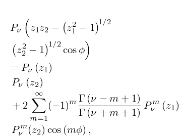
►Let $s$ be an arbitrary integer, and $P_{\nu }^{-\mu }\left(z{\mathrm{e}}^{s\pi \mathrm{i}}\right)$ and ${𝑸}_{\nu }^{\mu }\left(z{\mathrm{e}}^{s\pi \mathrm{i}}\right)$ denote the branches obtained from the principal branches by making $\frac{1}{2}s$ circuits, in the positive sense, of the ellipse having $\pm 1$ as foci and passing through $z$. … ►Next, let $P_{\nu ,s}^{-\mu }\left(z\right)$ and ${𝑸}_{\nu ,s}^{\mu }\left(z\right)$ denote the branches obtained from the principal branches by encircling the branch point $1$ (but not the branch point $-1$) $s$ times in the positive sense. … ►For fixed $z$, other than $\pm 1$ or $\mathrm{\infty }$, each branch of $P_{\nu }^{-\mu }\left(z\right)$ and ${𝑸}_{\nu }^{\mu }\left(z\right)$ is an entire function of each parameter $\nu$ and $\mu$. ►The behavior of $P_{\nu }^{-\mu }\left(z\right)$ and ${𝑸}_{\nu }^{\mu }\left(z\right)$ as $z\to -1$ from the left on the upper or lower side of the cut from $-\mathrm{\infty }$ to $1$ can be deduced from (14.8.7)–(14.8.11), combined with (14.24.1) and (14.24.2) with $s=\pm 1$.

19: 14.5 Special Values

… ►

14.5.5 $${𝖯}_0\left(x\right)=P_0\left(x\right)=1,$$

ⓘ

Symbols:

${𝖯}_{\nu }\left(x\right)={𝖯}_{\nu }^0\left(x\right)$: Ferrers function of the first kind, $P_{\nu }\left(z\right)=P_{\nu }^0\left(z\right)$: Legendre function of the first kind and $x$: real variable

A&S Ref:

8.4.1

Permalink:

http://dlmf.nist.gov/14.5.E5

Encodings:

pMML, png, TeX

See also:

Annotations for §14.5(ii), §14.5 and Ch.14

►

14.5.6 $${𝖯}_1\left(x\right)=P_1\left(x\right)=x.$$

ⓘ

Symbols:

${𝖯}_{\nu }\left(x\right)={𝖯}_{\nu }^0\left(x\right)$: Ferrers function of the first kind, $P_{\nu }\left(z\right)=P_{\nu }^0\left(z\right)$: Legendre function of the first kind and $x$: real variable

A&S Ref:

8.4.3

Permalink:

http://dlmf.nist.gov/14.5.E6

Encodings:

pMML, png, TeX

See also:

Annotations for §14.5(ii), §14.5 and Ch.14

… ►

§14.5(v) $\mu =0$, $\nu =\pm \frac{1}{2}$

… ► … ►

14.5.28 $${𝖯}_2\left(x\right)=P_2\left(x\right)=\frac{3x^2-1}{2},$$

ⓘ

Symbols:

${𝖯}_{\nu }\left(x\right)={𝖯}_{\nu }^0\left(x\right)$: Ferrers function of the first kind, $P_{\nu }\left(z\right)=P_{\nu }^0\left(z\right)$: Legendre function of the first kind and $x$: real variable

Referenced by:

(14.5.28)

Permalink:

http://dlmf.nist.gov/14.5.E28

Encodings:

pMML, png, TeX

Addition (effective with 1.0.7):

(14.5.28) has been added to this section.

See also:

Annotations for §14.5(vi), §14.5 and Ch.14

…

20: 14.17 Integrals

… ►In (14.17.1)–(14.17.4), $𝖯$ may be replaced by $𝖰$, and in (14.17.3) and (14.17.4), $𝖰$ may be replaced by $𝖯$. … ►

§14.17(iii) Orthogonality Properties

… ►Orthogonality relations for the associated Legendre functions of imaginary order are given in Bielski (2013). ►

§14.17(iv) Definite Integrals of Products

… ►

§14.17(v) Laplace Transforms

…