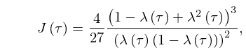
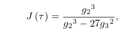
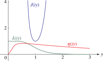
Klein complete invariant

SearchAdvancedHelp

(0.001 seconds)

6 matching pages

1: 23.19 Interrelations

… ►

23.19.2 $$J\left(\tau \right)=\frac{4}{27}\frac{{\left(1-\lambda \left(\tau \right)+{\lambda }^2\left(\tau \right)\right)}^3}{{\left(\lambda \left(\tau \right)\left(1-\lambda \left(\tau \right)\right)\right)}^2},$$

ⓘ

Symbols:

$J\left(\tau \right)$: Klein’s complete invariant, $\lambda \left(\tau \right)$: elliptic modular function and $\tau$: complex variable

Permalink:

http://dlmf.nist.gov/23.19.E2

Encodings:

pMML, png, TeX

See also:

Annotations for §23.19 and Ch.23

►

23.19.3 $$J\left(\tau \right)=\frac{g_2^3}{g_2^3-27g_3^2},$$

ⓘ

Symbols:

$J\left(\tau \right)$: Klein’s complete invariant, $g_j$: Weierstrass lattice invariants $g_2$, $g_3$ , $𝕃$: lattice and $\tau$: complex variable

Permalink:

http://dlmf.nist.gov/23.19.E3

Encodings:

pMML, png, TeX

See also:

Annotations for §23.19 and Ch.23

…

2: 23.15 Definitions

… ►

Klein’s Complete Invariant

►

23.15.7 $$J\left(\tau \right)=\frac{{\left({\theta }_2^8(0,q)+{\theta }_3^8(0,q)+{\theta }_4^8(0,q)\right)}^3}{54{\left({\theta }_1^{\prime }(0,q)\right)}^8},$$

ⓘ

Defines:

$J\left(\tau \right)$: Klein’s complete invariant

Symbols:

${\theta }_j(z,q)$: theta function, $q$: nome and $\tau$: complex variable

Permalink:

http://dlmf.nist.gov/23.15.E7

Encodings:

pMML, png, TeX

See also:

Annotations for §23.15(ii), §23.15(ii), §23.15 and Ch.23

…

3: 23.1 Special Notation

… ►The main functions treated in this chapter are the Weierstrass $\mathrm{\wp }$-function $\mathrm{\wp }\left(z\right)=\mathrm{\wp }\left(z|𝕃\right)=\mathrm{\wp }(z;g_2,g_3)$; the Weierstrass zeta function $\zeta \left(z\right)=\zeta \left(z|𝕃\right)=\zeta (z;g_2,g_3)$; the Weierstrass sigma function $\sigma \left(z\right)=\sigma \left(z|𝕃\right)=\sigma (z;g_2,g_3)$; the elliptic modular function $\lambda \left(\tau \right)$; Klein’s complete invariant $J\left(\tau \right)$; Dedekind’s eta function $\eta \left(\tau \right)$. …

4: 23.16 Graphics

… ►See Figures 23.16.1–23.16.3 for the modular functions $\lambda$, $J$, and $\eta$. … ►

►►

Figure 23.16.1: Modular functions $\lambda \left(\mathrm{i}y\right)$, $J\left(\mathrm{i}y\right)$, $\eta \left(\mathrm{i}y\right)$ for $0\le y\le 3$. … Magnify

…

5: 23.18 Modular Transformations

… ►

Klein’s Complete Invariant

►

23.18.4 $$J\left(𝒜\tau \right)=J\left(\tau \right).$$

ⓘ

Symbols:

$J\left(\tau \right)$: Klein’s complete invariant, $\tau$: complex variable and $𝒜$: bilinear transformation

Referenced by:

§23.18

Permalink:

http://dlmf.nist.gov/23.18.E4

Encodings:

pMML, png, TeX

See also:

Annotations for §23.18, §23.18 and Ch.23

…

6: 23.17 Elementary Properties

… ►

23.17.5 $$1728J\left(\tau \right)=q^{-2}+744+\mathrm{1\hspace{0.33em}96884}{q}^2+\mathrm{214\hspace{0.33em}93760}{q}^4+\mathrm{\cdots },$$

ⓘ

Symbols:

$J\left(\tau \right)$: Klein’s complete invariant, $q$: nome and $\tau$: complex variable

Referenced by:

§23.17(ii)

Permalink:

http://dlmf.nist.gov/23.17.E5

Encodings:

pMML, png, TeX

See also:

Annotations for §23.17(ii), §23.17 and Ch.23

…