Jacobi–Abel addition theorem

SearchAdvancedHelp

(0.003 seconds)

1—10 of 265 matching pages

1: 22.16 Related Functions

… ►

§22.16(i) Jacobi’s Amplitude ($\mathrm{am}$) Function

… ►

§22.16(ii) Jacobi’s Epsilon Function

… ►

Quasi-Addition and Quasi-Periodic Formulas

… ►

§22.16(iii) Jacobi’s Zeta Function

… ►

Properties

…

2: 18.3 Definitions

§18.3 Definitions

►The classical OP’s comprise the Jacobi, Laguerre and Hermite polynomials. … ►This table also includes the following special cases of Jacobi polynomials: ultraspherical, Chebyshev, and Legendre. … ►For finite power series of the Jacobi, ultraspherical, Laguerre, and Hermite polynomials, see §18.5(iii) (in powers of $x-1$ for Jacobi polynomials, in powers of $x$ for the other cases). … ►

Jacobi on Other Intervals

…

3: 22.18 Mathematical Applications

… ►

§22.18(iv) Elliptic Curves and the Jacobi–Abel Addition Theorem

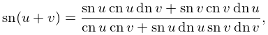
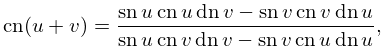
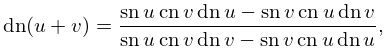
… ►For any two points $(x_1,y_1)$ and $(x_2,y_2)$ on this curve, their sum $(x_3,y_3)$, always a third point on the curve, is defined by the Jacobi–Abel addition law …a construction due to Abel; see Whittaker and Watson (1927, pp. 442, 496–497). …With the identification $x=\mathrm{sn}(z,k)$, $y=d(\mathrm{sn}(z,k))/dz$, the addition law (22.18.8) is transformed into the addition theorem (22.8.1); see Akhiezer (1990, pp. 42, 45, 73–74) and McKean and Moll (1999, §§2.14, 2.16). …

4: 22.8 Addition Theorems

§22.8 Addition Theorems

… ►

22.8.14 $$\mathrm{sn}(u+v)=\frac{\mathrm{sn}u\mathrm{cn}u\mathrm{dn}v+\mathrm{sn}v\mathrm{cn}v\mathrm{dn}u}{\mathrm{cn}u\mathrm{cn}v+\mathrm{sn}u\mathrm{dn}u\mathrm{sn}v\mathrm{dn}v},$$

ⓘ

Symbols:

$\mathrm{cn}(z,k)$: Jacobian elliptic function, $\mathrm{dn}(z,k)$: Jacobian elliptic function, $\mathrm{sn}(z,k)$: Jacobian elliptic function, $u$: complex, $v$: complex and $k$: modulus

Permalink:

http://dlmf.nist.gov/22.8.E14

Encodings:

pMML, png, TeX

See also:

Annotations for §22.8(ii), §22.8 and Ch.22

►

22.8.15 $$\mathrm{cn}(u+v)=\frac{\mathrm{sn}u\mathrm{cn}u\mathrm{dn}v-\mathrm{sn}v\mathrm{cn}v\mathrm{dn}u}{\mathrm{sn}u\mathrm{cn}v\mathrm{dn}v-\mathrm{sn}v\mathrm{cn}u\mathrm{dn}u},$$

ⓘ

Symbols:

$\mathrm{cn}(z,k)$: Jacobian elliptic function, $\mathrm{dn}(z,k)$: Jacobian elliptic function, $\mathrm{sn}(z,k)$: Jacobian elliptic function, $u$: complex, $v$: complex and $k$: modulus

Permalink:

http://dlmf.nist.gov/22.8.E15

Encodings:

pMML, png, TeX

See also:

Annotations for §22.8(ii), §22.8 and Ch.22

… ►

22.8.17 $$\mathrm{dn}(u+v)=\frac{\mathrm{sn}u\mathrm{cn}v\mathrm{dn}u-\mathrm{sn}v\mathrm{cn}u\mathrm{dn}v}{\mathrm{sn}u\mathrm{cn}v\mathrm{dn}v-\mathrm{sn}v\mathrm{cn}u\mathrm{dn}u},$$

ⓘ

Symbols:

$\mathrm{cn}(z,k)$: Jacobian elliptic function, $\mathrm{dn}(z,k)$: Jacobian elliptic function, $\mathrm{sn}(z,k)$: Jacobian elliptic function, $u$: complex, $v$: complex and $k$: modulus

Permalink:

http://dlmf.nist.gov/22.8.E17

Encodings:

pMML, png, TeX

See also:

Annotations for §22.8(ii), §22.8 and Ch.22

… ►

5: 28.27 Addition Theorems

§28.27 Addition Theorems

►Addition theorems provide important connections between Mathieu functions with different parameters and in different coordinate systems. They are analogous to the addition theorems for Bessel functions (§10.23(ii)) and modified Bessel functions (§10.44(ii)). …

6: 20.7 Identities

… ►

§20.7(ii) Addition Formulas

►

20.7.6 $${\theta }_4^2(0,q){\theta }_1(w+z,q){\theta }_1(w-z,q)={\theta }_3^2(w,q){\theta }_2^2(z,q)-{\theta }_2^2(w,q){\theta }_3^2(z,q),$$

ⓘ

Symbols:

${\theta }_j(z,q)$: theta function, $z$: complex and $q$: nome

Referenced by:

§20.7(ii)

Permalink:

http://dlmf.nist.gov/20.7.E6

Encodings:

pMML, png, TeX

See also:

Annotations for §20.7(ii), §20.7 and Ch.20

►

20.7.7 $${\theta }_4^2(0,q){\theta }_2(w+z,q){\theta }_2(w-z,q)={\theta }_4^2(w,q){\theta }_2^2(z,q)-{\theta }_1^2(w,q){\theta }_3^2(z,q),$$

ⓘ

Symbols:

${\theta }_j(z,q)$: theta function, $z$: complex and $q$: nome

Permalink:

http://dlmf.nist.gov/20.7.E7

Encodings:

pMML, png, TeX

See also:

Annotations for §20.7(ii), §20.7 and Ch.20

►

20.7.8 $${\theta }_4^2(0,q){\theta }_3(w+z,q){\theta }_3(w-z,q)={\theta }_4^2(w,q){\theta }_3^2(z,q)-{\theta }_1^2(w,q){\theta }_2^2(z,q),$$

ⓘ

Symbols:

${\theta }_j(z,q)$: theta function, $z$: complex and $q$: nome

Permalink:

http://dlmf.nist.gov/20.7.E8

Encodings:

pMML, png, TeX

See also:

Annotations for §20.7(ii), §20.7 and Ch.20

… ►

20.7.10 $${\theta }_1(2z,q)=2\frac{{\theta }_1(z,q){\theta }_2(z,q){\theta }_3(z,q){\theta }_4(z,q)}{{\theta }_2(0,q){\theta }_3(0,q){\theta }_4(0,q)}.$$

ⓘ

Symbols:

${\theta }_j(z,q)$: theta function, $z$: complex and $q$: nome

Permalink:

http://dlmf.nist.gov/20.7.E10

Encodings:

pMML, png, TeX

See also:

Annotations for §20.7(iii), §20.7 and Ch.20

…

7: 20.11 Generalizations and Analogs

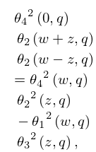
… ►This is Jacobi’s inversion problem of §20.9(ii). … ►Each provides an extension of Jacobi’s inversion problem. … ►For $m=1,2,3,4$, $n=1,2,3,4$, and $m\ne n$, define twelve combined theta functions ${\phi }_{m,n}(z,q)$ by … ►Such sets of twelve equations include derivatives, differential equations, bisection relations, duplication relations, addition formulas (including new ones for theta functions), and pseudo-addition formulas. …

8: 18.14 Inequalities

… ►

Jacobi

… ►

Jacobi

… ►

Jacobi

… ►

Szegő–Szász Inequality

… ►

Jacobi

…

9: 18.18 Sums

… ►

Jacobi

… ►

§18.18(ii) Addition Theorems

►

Ultraspherical

… ►

Legendre

… ►

Jacobi

…

10: 14.28 Sums

… ►

§14.28(i) Addition Theorem

… ►For generalizations in terms of Gegenbauer and Jacobi polynomials, see Theorem 2. 1 in Cohl (2013b) and Theorem 1 in Cohl (2013a) respectively. …