Coulomb potential barriers

SearchAdvancedHelp

(0.002 seconds)

11—20 of 78 matching pages

11: 33.3 Graphics

§33.3 Graphics

►

§33.3(i) Line Graphs of the Coulomb Radial Functions $F_{\mathrm{\ell }}(\eta ,\rho )$ and $G_{\mathrm{\ell }}(\eta ,\rho )$

… ►

►►

Figure 33.3.3: $F_{\mathrm{\ell }}(\eta ,\rho )$, $G_{\mathrm{\ell }}(\eta ,\rho )$ with $\mathrm{\ell }=0$, $\eta =2$. The turning point is at ${\rho }_{\mathrm{tp}}(2,0)=4$. Magnify

… ►

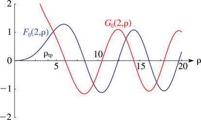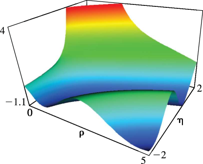
§33.3(ii) Surfaces of the Coulomb Radial Functions $F_0(\eta ,\rho )$ and $G_0(\eta ,\rho )$

… ►

►

►

Figure 33.3.8: $G_0(\eta ,\rho )$, $-2\le \eta \le 2$, . Magnify 3D Help

12: 18.39 Applications in the Physical Sciences

… ►

The Quantum Coulomb Problem

… ►This is Coulomb’s Law. … ►

The Relativistic Quantum Coulomb Problem

… ►The positive energy (scattering) eigenfunctions for the above Coulomb problem, with potential $V(r)=-Z{e}^2/r$ are discussed in Chapter 33 for each integer $l$. … ►

The Coulomb–Pollaczek Polynomials

…

13: 33.18 Limiting Forms for Large $\mathrm{\ell }$

§33.18 Limiting Forms for Large $\mathrm{\ell }$

… ►

$f(ϵ,\mathrm{\ell };r)\sim {\displaystyle \frac{{(2r)}^{\mathrm{\ell }+1}}{(2\mathrm{\ell }+1)!}},$

►

$h(ϵ,\mathrm{\ell };r)\sim {\displaystyle \frac{(2\mathrm{\ell })!}{\pi {(2r)}^{\mathrm{\ell }}}}.$

14: 33.24 Tables

§33.24 Tables

►

Abramowitz and Stegun (1964, Chapter 14) tabulates $F_0(\eta ,\rho )$, $G_0(\eta ,\rho )$, $F_0^{\prime }(\eta ,\rho )$, and $G_0^{\prime }(\eta ,\rho )$ for $\eta =0.5(.5)20$ and $\rho =1(1)20$, 5S; $C_0\left(\eta \right)$ for $\eta =0(.05)3$, 6S.

…

15: 33.1 Special Notation

… ►The main functions treated in this chapter are first the Coulomb radial functions $F_{\mathrm{\ell }}(\eta ,\rho )$, $G_{\mathrm{\ell }}(\eta ,\rho )$, $H_{\mathrm{\ell }}^{\pm }(\eta ,\rho )$ (Sommerfeld (1928)), which are used in the case of repulsive Coulomb interactions, and secondly the functions $f(ϵ,\mathrm{\ell };r)$, $h(ϵ,\mathrm{\ell };r)$, $s(ϵ,\mathrm{\ell };r)$, $c(ϵ,\mathrm{\ell };r)$ (Seaton (1982, 2002a)), which are used in the case of attractive Coulomb interactions. … ►

$P_{\mathrm{\ell }}(ϵ,r)=(2\mathrm{\ell }+1)!f(ϵ,\mathrm{\ell };r)/2^{\mathrm{\ell }+1}$, $Q_{\mathrm{\ell }}(ϵ,r)=-(2\mathrm{\ell }+1)!h(ϵ,\mathrm{\ell };r)/(2^{\mathrm{\ell }+1}A(ϵ,\mathrm{\ell }))$.

►

$f^{(0)}(ϵ,\mathrm{\ell };r)=f(ϵ,\mathrm{\ell };r)$, $f(ϵ,\mathrm{\ell };r)=s(ϵ,\mathrm{\ell };r)$, $g(ϵ,\mathrm{\ell };r)=c(ϵ,\mathrm{\ell };r)$.

16: 33.13 Complex Variable and Parameters

§33.13 Complex Variable and Parameters

►The functions $F_{\mathrm{\ell }}(\eta ,\rho )$, $G_{\mathrm{\ell }}(\eta ,\rho )$, and $H_{\mathrm{\ell }}^{\pm }(\eta ,\rho )$ may be extended to noninteger values of $\mathrm{\ell }$ by generalizing $(2\mathrm{\ell }+1)!=\mathrm{\Gamma }\left(2\mathrm{\ell }+2\right)$, and supplementing (33.6.5) by a formula derived from (33.2.8) with $U(a,b,z)$ expanded via (13.2.42). … ►The quantities $C_{\mathrm{\ell }}\left(\eta \right)$, ${\sigma }_{\mathrm{\ell }}\left(\eta \right)$, and $R_{\mathrm{\ell }}$, given by (33.2.6), (33.2.10), and (33.4.1), respectively, must be defined consistently so that ►

33.13.1 $$C_{\mathrm{\ell }}\left(\eta \right)=2^{\mathrm{\ell }}{\mathrm{e}}^{\mathrm{i}{\sigma }_{\mathrm{\ell }}\left(\eta \right)-(\pi \eta /2)}\mathrm{\Gamma }\left(\mathrm{\ell }+1-\mathrm{i}\eta \right)/\mathrm{\Gamma }\left(2\mathrm{\ell }+2\right),$$

ⓘ

Symbols:

$C_{\mathrm{\ell }}\left(\eta \right)$: normalizing constant for Coulomb radial functions, ${\sigma }_{\mathrm{\ell }}\left(\eta \right)$: Coulomb phase shift, $\mathrm{\Gamma }\left(z\right)$: gamma function, $\pi$: the ratio of the circumference of a circle to its diameter, $\mathrm{e}$: base of natural logarithm, $\mathrm{i}$: imaginary unit, $\mathrm{\ell }$: nonnegative integer and $\eta$: real parameter

Permalink:

http://dlmf.nist.gov/33.13.E1

Encodings:

pMML, png, TeX

See also:

Annotations for §33.13 and Ch.33

… ►

33.13.2 $$R_{\mathrm{\ell }}=(2\mathrm{\ell }+1)C_{\mathrm{\ell }}\left(\eta \right)/C_{\mathrm{\ell }-1}\left(\eta \right).$$

ⓘ

Symbols:

$C_{\mathrm{\ell }}\left(\eta \right)$: normalizing constant for Coulomb radial functions, $\mathrm{\ell }$: nonnegative integer, $\eta$: real parameter and $R_{\mathrm{\ell }}$: factor

Permalink:

http://dlmf.nist.gov/33.13.E2

Encodings:

pMML, png, TeX

See also:

Annotations for §33.13 and Ch.33

…

17: 33.14 Definitions and Basic Properties

… ►

§33.14(i) Coulomb Wave Equation

… ►

§33.14(ii) Regular Solution $f(ϵ,\mathrm{\ell };r)$

… ►

§33.14(iii) Irregular Solution $h(ϵ,\mathrm{\ell };r)$

… ►

§33.14(iv) Solutions $s(ϵ,\mathrm{\ell };r)$ and $c(ϵ,\mathrm{\ell };r)$

… ►

§33.14(v) Wronskians

…

18: 33.5 Limiting Forms for Small $\rho$, Small $|\eta |$, or Large $\mathrm{\ell }$

… ►

§33.5(i) Small $\rho$

… ►

$F_{\mathrm{\ell }}(\eta ,\rho )\sim C_{\mathrm{\ell }}\left(\eta \right){\rho }^{\mathrm{\ell }+1},$

… ►

§33.5(ii) $\eta =0$

… ►

§33.5(iii) Small $|\eta |$

… ►

§33.5(iv) Large $\mathrm{\ell }$

…

19: 33.23 Methods of Computation

§33.23 Methods of Computation

… ►The methods used for computing the Coulomb functions described below are similar to those in §13.29. … ►Combined with the Wronskians (33.2.12), the values of $F_{\mathrm{\ell }}$, $G_{\mathrm{\ell }}$, and their derivatives can be extracted. … ►

§33.23(vii) WKBJ Approximations

… ►Hull and Breit (1959) and Barnett (1981b) give WKBJ approximations for $F_0$ and $G_0$ in the region inside the turning point: .

20: 33.8 Continued Fractions

§33.8 Continued Fractions

… ►If we denote $u=F_{\mathrm{\ell }}^{\prime }/F_{\mathrm{\ell }}$ and $p+\mathrm{i}q=H_{\mathrm{\ell }}^{+}{}_{}{}^{\prime }/H_{\mathrm{\ell }}^{+}$, then … ►

$F_{\mathrm{\ell }}^{\prime }=u{F}_{\mathrm{\ell }},$

►

$G_{\mathrm{\ell }}=q^{-1}(u-p)F_{\mathrm{\ell }},$

►

$G_{\mathrm{\ell }}^{\prime }=q^{-1}(up-p^2-q^2)F_{\mathrm{\ell }}.$

…