Coulomb excitation of nuclei

SearchAdvancedHelp

(0.001 seconds)

1—10 of 62 matching pages

1: 33.22 Particle Scattering and Atomic and Molecular Spectra

… ►

§33.22(i) Schrödinger Equation

… ► ►►

Attractive potentials:	, .
…

►Positive-energy functions correspond to processes such as Rutherford scattering and Coulomb excitation of nuclei (Alder et al. (1956)), and atomic photo-ionization and electron-ion collisions (Bethe and Salpeter (1977)). … ► … ►

§33.22(iv) Klein–Gordon and Dirac Equations

…

2: Bibliography B

… ►

The attractive Coulomb potential polynomials. Constr. Approx. 1 (2), pp. 103–119.

ⓘ

External Links:

ISSN 0176-4276, Document, Link, MathReview (W. A. Al-Salam)

Referenced by:

§18.39(iv), §18.39(iv).

Encodings:

BibTeX

… ►

An algorithm for regular and irregular Coulomb and Bessel functions of real order to machine accuracy. Comput. Phys. Comm. 21 (3), pp. 297–314.

ⓘ

External Links:

Document

Referenced by:

§3.10(iii), §33.22(iv).

Encodings:

BibTeX

… ►

Coulomb functions (negative energies). Comput. Phys. Comm. 20 (3), pp. 447–458.

ⓘ

Notes:

Double-precision Fortran code.

External Links:

Document, Code

Referenced by:

1st item, 4th item.

Encodings:

BibTeX

… ►

Quasinormal ringing of Kerr black holes: The excitation factors. Phys. Rev. D 74 (104020), pp. 1–27.

ⓘ

External Links:

ISSN 0556-2821, Document, MathReview

Referenced by:

6th item.

Encodings:

BibTeX

… ►

Coulomb functions for reactions of protons and alpha-particles with the lighter nuclei. Rev. Modern Physics 23 (2), pp. 147–182.

ⓘ

External Links:

ISSN 0034-6861, Document, MathReview (A. Erdélyi), ZentralBlatt

Referenced by:

§33.22(v).

Encodings:

BibTeX

…

3: 33.17 Recurrence Relations and Derivatives

§33.17 Recurrence Relations and Derivatives

►

33.17.1 $$(\mathrm{\ell }+1)rf(ϵ,\mathrm{\ell }-1;r)-(2\mathrm{\ell }+1)\left(\mathrm{\ell }(\mathrm{\ell }+1)-r\right)f(ϵ,\mathrm{\ell };r)+\mathrm{\ell }\left(1+{(\mathrm{\ell }+1)}^2ϵ\right)rf(ϵ,\mathrm{\ell }+1;r)=0,$$

ⓘ

Symbols:

$f(ϵ,\mathrm{\ell };r)$: regular Coulomb function, $\mathrm{\ell }$: nonnegative integer, $r$: real variable and $ϵ$: real parameter

Permalink:

http://dlmf.nist.gov/33.17.E1

Encodings:

pMML, png, TeX

See also:

Annotations for §33.17 and Ch.33

►

33.17.2 $$(\mathrm{\ell }+1)\left(1+{\mathrm{\ell }}^2ϵ\right)rh(ϵ,\mathrm{\ell }-1;r)-(2\mathrm{\ell }+1)\left(\mathrm{\ell }(\mathrm{\ell }+1)-r\right)h(ϵ,\mathrm{\ell };r)+\mathrm{\ell }rh(ϵ,\mathrm{\ell }+1;r)=0,$$

ⓘ

Symbols:

$h(ϵ,\mathrm{\ell };r)$: irregular Coulomb function, $\mathrm{\ell }$: nonnegative integer, $r$: real variable and $ϵ$: real parameter

Permalink:

http://dlmf.nist.gov/33.17.E2

Encodings:

pMML, png, TeX

See also:

Annotations for §33.17 and Ch.33

►

33.17.3 $$(\mathrm{\ell }+1)r{f}^{\prime }(ϵ,\mathrm{\ell };r)=\left({(\mathrm{\ell }+1)}^2-r\right)f(ϵ,\mathrm{\ell };r)-\left(1+{(\mathrm{\ell }+1)}^2ϵ\right)rf(ϵ,\mathrm{\ell }+1;r),$$

ⓘ

Symbols:

$f(ϵ,\mathrm{\ell };r)$: regular Coulomb function, $\mathrm{\ell }$: nonnegative integer, $r$: real variable and $ϵ$: real parameter

Permalink:

http://dlmf.nist.gov/33.17.E3

Encodings:

pMML, png, TeX

See also:

Annotations for §33.17 and Ch.33

►

33.17.4 $$(\mathrm{\ell }+1)r{h}^{\prime }(ϵ,\mathrm{\ell };r)=\left({(\mathrm{\ell }+1)}^2-r\right)h(ϵ,\mathrm{\ell };r)-rh(ϵ,\mathrm{\ell }+1;r).$$

ⓘ

Symbols:

$h(ϵ,\mathrm{\ell };r)$: irregular Coulomb function, $\mathrm{\ell }$: nonnegative integer, $r$: real variable and $ϵ$: real parameter

Permalink:

http://dlmf.nist.gov/33.17.E4

Encodings:

pMML, png, TeX

See also:

Annotations for §33.17 and Ch.33

4: 33.15 Graphics

§33.15 Graphics

►

§33.15(i) Line Graphs of the Coulomb Functions $f(ϵ,\mathrm{\ell };r)$ and $h(ϵ,\mathrm{\ell };r)$

►

►►

Figure 33.15.1: $f(ϵ,\mathrm{\ell };r),h(ϵ,\mathrm{\ell };r)$ with $\mathrm{\ell }=0,ϵ=4$. Magnify

… ►

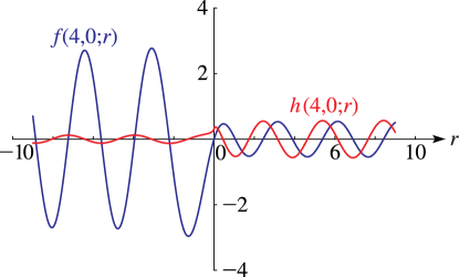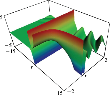
§33.15(ii) Surfaces of the Coulomb Functions $f(ϵ,\mathrm{\ell };r)$, $h(ϵ,\mathrm{\ell };r)$, $s(ϵ,\mathrm{\ell };r)$, and $c(ϵ,\mathrm{\ell };r)$

… ►

►

►

Figure 33.15.9: $h(ϵ,\mathrm{\ell };r)$ with . Magnify 3D Help

…

5: 33.2 Definitions and Basic Properties

… ►

§33.2(i) Coulomb Wave Equation

… ►The functions $H_{\mathrm{\ell }}^{\pm }(\eta ,\rho )$ are defined by …${\sigma }_{\mathrm{\ell }}\left(\eta \right)$ is the Coulomb phase shift. … ►

§33.2(iv) Wronskians and Cross-Product

…

6: 33.3 Graphics

§33.3 Graphics

►

§33.3(i) Line Graphs of the Coulomb Radial Functions $F_{\mathrm{\ell }}(\eta ,\rho )$ and $G_{\mathrm{\ell }}(\eta ,\rho )$

… ►

►►

Figure 33.3.3: $F_{\mathrm{\ell }}(\eta ,\rho )$, $G_{\mathrm{\ell }}(\eta ,\rho )$ with $\mathrm{\ell }=0$, $\eta =2$. The turning point is at ${\rho }_{\mathrm{tp}}(2,0)=4$. Magnify

… ►

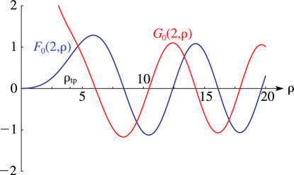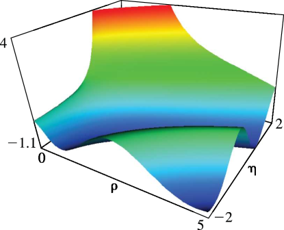
§33.3(ii) Surfaces of the Coulomb Radial Functions $F_0(\eta ,\rho )$ and $G_0(\eta ,\rho )$

… ►

►

►

Figure 33.3.8: $G_0(\eta ,\rho )$, $-2\le \eta \le 2$, . Magnify 3D Help

7: 33.18 Limiting Forms for Large $\mathrm{\ell }$

§33.18 Limiting Forms for Large $\mathrm{\ell }$

… ►

$f(ϵ,\mathrm{\ell };r)\sim {\displaystyle \frac{{(2r)}^{\mathrm{\ell }+1}}{(2\mathrm{\ell }+1)!}},$

►

$h(ϵ,\mathrm{\ell };r)\sim {\displaystyle \frac{(2\mathrm{\ell })!}{\pi {(2r)}^{\mathrm{\ell }}}}.$

8: 33.24 Tables

§33.24 Tables

►

Abramowitz and Stegun (1964, Chapter 14) tabulates $F_0(\eta ,\rho )$, $G_0(\eta ,\rho )$, $F_0^{\prime }(\eta ,\rho )$, and $G_0^{\prime }(\eta ,\rho )$ for $\eta =0.5(.5)20$ and $\rho =1(1)20$, 5S; $C_0\left(\eta \right)$ for $\eta =0(.05)3$, 6S.

…

9: 18.39 Applications in the Physical Sciences

… ►

The Quantum Coulomb Problem

… ►This is Coulomb’s Law. … ►

c) Spherical Radial Coulomb Wave Functions

… ►

The Relativistic Quantum Coulomb Problem

… ►

The Coulomb–Pollaczek Polynomials

…

10: 33.1 Special Notation

… ►The main functions treated in this chapter are first the Coulomb radial functions $F_{\mathrm{\ell }}(\eta ,\rho )$, $G_{\mathrm{\ell }}(\eta ,\rho )$, $H_{\mathrm{\ell }}^{\pm }(\eta ,\rho )$ (Sommerfeld (1928)), which are used in the case of repulsive Coulomb interactions, and secondly the functions $f(ϵ,\mathrm{\ell };r)$, $h(ϵ,\mathrm{\ell };r)$, $s(ϵ,\mathrm{\ell };r)$, $c(ϵ,\mathrm{\ell };r)$ (Seaton (1982, 2002a)), which are used in the case of attractive Coulomb interactions. … ►

$P_{\mathrm{\ell }}(ϵ,r)=(2\mathrm{\ell }+1)!f(ϵ,\mathrm{\ell };r)/2^{\mathrm{\ell }+1}$, $Q_{\mathrm{\ell }}(ϵ,r)=-(2\mathrm{\ell }+1)!h(ϵ,\mathrm{\ell };r)/(2^{\mathrm{\ell }+1}A(ϵ,\mathrm{\ell }))$.

►

$f^{(0)}(ϵ,\mathrm{\ell };r)=f(ϵ,\mathrm{\ell };r)$, $f(ϵ,\mathrm{\ell };r)=s(ϵ,\mathrm{\ell };r)$, $g(ϵ,\mathrm{\ell };r)=c(ϵ,\mathrm{\ell };r)$.