About the Project
13 Confluent Hypergeometric FunctionsKummer Functions

§13.4 Integral Representations

Contents
  1. §13.4(i) Integrals Along the Real Line
  2. §13.4(ii) Contour Integrals
  3. §13.4(iii) Mellin–Barnes Integrals

§13.4(i) Integrals Along the Real Line

13.4.1 𝐌⁡(a,b,z)=1Γ⁡(a)⁢Γ⁡(b−a)⁢∫01ez⁢t⁢ta−1⁢(1−t)b−a−1⁢dt,
ℜ⁡b>ℜ⁡a>0,
13.4.2 𝐌⁡(a,b,z)=1Γ⁡(b−c)⁢∫01𝐌⁡(a,c,z⁢t)⁢tc−1⁢(1−t)b−c−1⁢dt,
ℜ⁡b>ℜ⁡c>0,
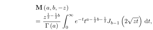
13.4.3 𝐌⁡(a,b,−z)=z12−12⁢bΓ⁡(a)⁢∫0∞e−t⁢ta−12⁢b−12⁢Jb−1⁡(2⁢z⁢t)⁢dt,
ℜ⁡a>0.

For the function Jb−1 see §10.2(ii).

13.4.4 U⁡(a,b,z)=1Γ⁡(a)⁢∫0∞e−z⁢t⁢ta−1⁢(1+t)b−a−1⁢dt,
ℜ⁡a>0, |ph⁡z|<12⁢π,
13.4.5 U⁡(a,b,z)=z1−aΓ⁡(a)⁢Γ⁡(1+a−b)⁢∫0∞U⁡(b−a,b,t)⁢e−t⁢ta−1t+z⁢dt,
|ph⁡z|<π, ℜ⁡a>max⁡(ℜ⁡b−1,0),
13.4.6 U⁡(a,b,z)=(−1)n⁢z1−b−nΓ⁡(1+a−b)⁢∫0∞𝐌⁡(b−a,b,t)⁢e−t⁢tb+n−1t+z⁢dt,
|ph⁡z|<π, n=0,1,2,…, −ℜ⁡b<n<1+ℜ⁡(a−b),
13.4.7 U⁡(a,b,z)=2⁢z12−12⁢bΓ⁡(a)⁢Γ⁡(a−b+1)⁢∫0∞e−t⁢ta−12⁢b−12⁢Kb−1⁡(2⁢z⁢t)⁢dt,
ℜ⁡a>max⁡(ℜ⁡b−1,0),
13.4.8 U⁡(a,b,z)=zc−a⁢∫0∞e−z⁢t⁢tc−1⁢𝐅12⁡(a,a−b+1;c;−t)⁢dt,
|ph⁡z|<12⁢π,

where c is arbitrary, ℜ⁡c>0. For the functions Kb−1 and 𝐅12 see §10.25(ii) and §§15.1, 15.2(i).

§13.4(ii) Contour Integrals

13.4.9 𝐌⁡(a,b,z)=Γ⁡(1+a−b)2⁢π⁢i⁢Γ⁡(a)⁢∫0(1+)ez⁢t⁢ta−1⁢(t−1)b−a−1⁢dt,
b−a≠1,2,3,…, ℜ⁡a>0.
13.4.10 𝐌⁡(a,b,z)=e−a⁢π⁢i⁢Γ⁡(1−a)2⁢π⁢i⁢Γ⁡(b−a)⁢∫1(0+)ez⁢t⁢ta−1⁢(1−t)b−a−1⁢dt,
a≠1,2,3,…, ℜ⁡(b−a)>0.
See accompanying text
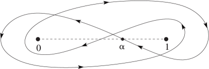
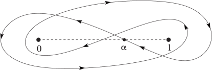
Figure 13.4.1: Contour of integration in (13.4.11). (Compare Figure 5.12.3.) Magnify
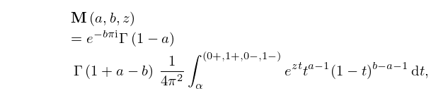
13.4.11 𝐌⁡(a,b,z)=e−b⁢π⁢i⁢Γ⁡(1−a)⁢Γ⁡(1+a−b)⁢14⁢π2×∫α(0+,1+,0−,1−)ez⁢t⁢ta−1⁢(1−t)b−a−1⁢dt,
a,b−a≠1,2,3,….

The contour of integration starts and terminates at a point α on the real axis between 0 and 1. It encircles t=0 and t=1 once in the positive sense, and then once in the negative sense. See Figure 13.4.1. The fractional powers are continuous and assume their principal values at t=α. Similar conventions also apply to the remaining integrals in this subsection.

13.4.12 𝐌⁡(a,c,z)=Γ⁡(b)2⁢π⁢i⁢z1−b⁢∫−∞(0+,1+)ez⁢t⁢t−b⁢𝐅12⁡(a,b;c;1/t)⁢dt,
b≠0,−1,−2,…, |ph⁡z|<12⁢π.

At the point where the contour crosses the interval (1,∞), t−b and the 𝐅12 function assume their principal values; compare §§15.1 and 15.2(i). A special case is

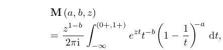
13.4.13 𝐌⁡(a,b,z)=z1−b2⁢π⁢i⁢∫−∞(0+,1+)ez⁢t⁢t−b⁢(1−1t)−a⁢dt,
|ph⁡z|<12⁢π.
13.4.14 U⁡(a,b,z)=e−a⁢π⁢i⁢Γ⁡(1−a)2⁢π⁢i⁢∫∞(0+)e−z⁢t⁢ta−1⁢(1+t)b−a−1⁢dt,
a≠1,2,3,…, |ph⁡z|<12⁢π.

The contour cuts the real axis between −1 and 0. At this point the fractional powers are determined by ph⁡t=π and ph⁡(1+t)=0.

Again, t−c and the 𝐅12 function assume their principal values where the contour (see Figure 5.9.1) intersects the positive real axis.

§13.4(iii) Mellin–Barnes Integrals

If a≠0,−1,−2,…, then

13.4.16 𝐌⁡(a,b,−z)=12⁢π⁢i⁢Γ⁡(a)⁢∫−i⁢∞i⁢∞Γ⁡(a+t)⁢Γ⁡(−t)Γ⁡(b+t)⁢zt⁢dt,
|ph⁡z|<12⁢π,

where the contour of integration separates the poles of Γ⁡(a+t) from those of Γ⁡(−t).

If a and a−b+1≠0,−1,−2,…, then

13.4.17 U⁡(a,b,z)=z−a2⁢π⁢i⁢∫−i⁢∞i⁢∞Γ⁡(a+t)⁢Γ⁡(1+a−b+t)⁢Γ⁡(−t)Γ⁡(a)⁢Γ⁡(1+a−b)⁢z−t⁢dt,
|ph⁡z|<32⁢π,

where the contour of integration separates the poles of Γ⁡(a+t)⁢Γ⁡(1+a−b+t) from those of Γ⁡(−t).

13.4.18 U⁡(a,b,z)=z1−b⁢ez2⁢π⁢i⁢∫−i⁢∞i⁢∞Γ⁡(b−1+t)⁢Γ⁡(t)Γ⁡(a+t)⁢z−t⁢dt,
|ph⁡z|<12⁢π,

where the contour of integration passes all the poles of Γ⁡(b−1+t)⁢Γ⁡(t) on the right-hand side.