推排九扑克牌咋玩【杏彩体育qee9.com】3cN

SearchAdvancedHelp

The term"qee9.com" was not found.Possible alternative term: "becom".

(0.001 seconds)

1—10 of 579 matching pages

1: 34.2 Definition: $\mathit{3}j$ Symbol

§34.2 Definition: $\mathit{3}j$ Symbol

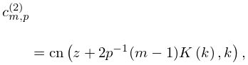
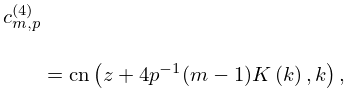
►The quantities $j_1,j_2,j_3$ in the $\mathit{3}j$ symbol are called angular momenta. …They therefore satisfy the triangle conditions …where $r,s,t$ is any permutation of $1,2,3$. The corresponding projective quantum numbers $m_1,m_2,m_3$ are given by …

2: 22.8 Addition Theorems

… ►

22.8.15 $$\mathrm{cn}(u+v)=\frac{\mathrm{sn}u\mathrm{cn}u\mathrm{dn}v-\mathrm{sn}v\mathrm{cn}v\mathrm{dn}u}{\mathrm{sn}u\mathrm{cn}v\mathrm{dn}v-\mathrm{sn}v\mathrm{cn}u\mathrm{dn}u},$$

ⓘ

Symbols:

$\mathrm{cn}(z,k)$: Jacobian elliptic function, $\mathrm{dn}(z,k)$: Jacobian elliptic function, $\mathrm{sn}(z,k)$: Jacobian elliptic function, $u$: complex, $v$: complex and $k$: modulus

Permalink:

http://dlmf.nist.gov/22.8.E15

Encodings:

pMML, png, TeX

See also:

Annotations for §22.8(ii), §22.8 and Ch.22

… ►

22.8.20

ⓘ

Symbols:

$\mathrm{cn}(z,k)$: Jacobian elliptic function, $\mathrm{dn}(z,k)$: Jacobian elliptic function, $\mathrm{sn}(z,k)$: Jacobian elliptic function, $det$: determinant, $z$: complex and $k$: modulus

Referenced by:

§22.8(iii)

Permalink:

http://dlmf.nist.gov/22.8.E20

Encodings:

pMML, png, TeX

See also:

Annotations for §22.8(iii), §22.8 and Ch.22

… ►

22.8.21 $$k_{}^{\prime }{}_{}{}^2-k_{}^{\prime }{}_{}{}^2{k}^2\mathrm{sn}{z}_1\mathrm{sn}{z}_2\mathrm{sn}{z}_3\mathrm{sn}{z}_4+k^2\mathrm{cn}{z}_1\mathrm{cn}{z}_2\mathrm{cn}{z}_3\mathrm{cn}{z}_4-\mathrm{dn}{z}_1\mathrm{dn}{z}_2\mathrm{dn}{z}_3\mathrm{dn}{z}_4=0.$$

ⓘ

Symbols:

$\mathrm{cn}(z,k)$: Jacobian elliptic function, $\mathrm{dn}(z,k)$: Jacobian elliptic function, $\mathrm{sn}(z,k)$: Jacobian elliptic function, $z$: complex, $k$: modulus and $k^{\prime }$: complementary modulus

Permalink:

http://dlmf.nist.gov/22.8.E21

Encodings:

pMML, png, TeX

See also:

Annotations for §22.8(iii), §22.8 and Ch.22

… ►

22.8.23

ⓘ

Symbols:

$\mathrm{cn}(z,k)$: Jacobian elliptic function, $\mathrm{dn}(z,k)$: Jacobian elliptic function, $\mathrm{sn}(z,k)$: Jacobian elliptic function, $det$: determinant, $z$: complex and $k$: modulus

Permalink:

http://dlmf.nist.gov/22.8.E23

Encodings:

pMML, png, TeX

See also:

Annotations for §22.8(iii), §22.8 and Ch.22

… ►is independent of $z_1$, $z_2$, $z_3$. …

3: 22.18 Mathematical Applications

… ►

$y=b\mathrm{cn}(u,k),$

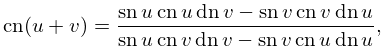
… ►By use of the functions $\mathrm{sn}$ and $\mathrm{cn}$, parametrizations of algebraic equations, such as … ►Algebraic curves of the form $y^2=P(x)$, where $P$ is a nonsingular polynomial of degree 3 or 4 (see McKean and Moll (1999, §1.10)), are elliptic curves, which are also considered in §23.20(ii). …For any two points $(x_1,y_1)$ and $(x_2,y_2)$ on this curve, their sum $(x_3,y_3)$, always a third point on the curve, is defined by the Jacobi–Abel addition law …This provides an abelian group structure, and leads to important results in number theory, discussed in an elementary manner by Silverman and Tate (1992), and more fully by Koblitz (1993, Chapter 1, especially §1.7) and McKean and Moll (1999, Chapter 3). …

4: 22.13 Derivatives and Differential Equations

… ►

22.13.2 $${\left(\frac{d}{dz}\mathrm{cn}(z,k)\right)}^2=\left(1-{\mathrm{cn}}^2(z,k)\right)\left(k_{}^{\prime }{}_{}{}^2+k^2{\mathrm{cn}}^2(z,k)\right),$$

ⓘ

Symbols:

$\mathrm{cn}(z,k)$: Jacobian elliptic function, $\frac{df}{dx}$: derivative of $f$ with respect to $x$ , $z$: complex, $k$: modulus and $k^{\prime }$: complementary modulus

Permalink:

http://dlmf.nist.gov/22.13.E2

Encodings:

pMML, png, TeX

See also:

Annotations for §22.13(ii), §22.13 and Ch.22

… ►

22.13.13 $$\frac{d^2}{{dz}^2}\mathrm{sn}(z,k)=-(1+k^2)\mathrm{sn}(z,k)+2k^2{\mathrm{sn}}^3(z,k),$$

ⓘ

Symbols:

$\mathrm{sn}(z,k)$: Jacobian elliptic function, $\frac{df}{dx}$: derivative of $f$ with respect to $x$ , $z$: complex and $k$: modulus

Referenced by:

§22.10(i), §22.10(ii), §22.13(iii)

Permalink:

http://dlmf.nist.gov/22.13.E13

Encodings:

pMML, png, TeX

See also:

Annotations for §22.13(iii), §22.13 and Ch.22

►

22.13.14 $$\frac{d^2}{{dz}^2}\mathrm{cn}(z,k)=-(k_{}^{\prime }{}_{}{}^2-k^2)\mathrm{cn}(z,k)-2k^2{\mathrm{cn}}^3(z,k),$$

ⓘ

Symbols:

$\mathrm{cn}(z,k)$: Jacobian elliptic function, $\frac{df}{dx}$: derivative of $f$ with respect to $x$ , $z$: complex, $k$: modulus and $k^{\prime }$: complementary modulus

Referenced by:

§22.10(i), §22.10(ii)

Permalink:

http://dlmf.nist.gov/22.13.E14

Encodings:

pMML, png, TeX

See also:

Annotations for §22.13(iii), §22.13 and Ch.22

►

22.13.15 $$\frac{d^2}{{dz}^2}\mathrm{dn}(z,k)=(1+k_{}^{\prime }{}_{}{}^2)\mathrm{dn}(z,k)-2{\mathrm{dn}}^3(z,k).$$

ⓘ

Symbols:

$\mathrm{dn}(z,k)$: Jacobian elliptic function, $\frac{df}{dx}$: derivative of $f$ with respect to $x$ , $z$: complex, $k$: modulus and $k^{\prime }$: complementary modulus

Referenced by:

§22.10(i), §22.10(ii)

Permalink:

http://dlmf.nist.gov/22.13.E15

Encodings:

pMML, png, TeX

See also:

Annotations for §22.13(iii), §22.13 and Ch.22

►

22.13.16 $$\frac{d^2}{{dz}^2}\mathrm{cd}(z,k)=-(1+k^2)\mathrm{cd}(z,k)+2k^2{\mathrm{cd}}^3(z,k),$$

ⓘ

Symbols:

$\mathrm{cd}(z,k)$: Jacobian elliptic function, $\frac{df}{dx}$: derivative of $f$ with respect to $x$ , $z$: complex and $k$: modulus

Permalink:

http://dlmf.nist.gov/22.13.E16

Encodings:

pMML, png, TeX

See also:

Annotations for §22.13(iii), §22.13 and Ch.22

…

5: 22.10 Maclaurin Series

… ►

22.10.1 $$\mathrm{sn}(z,k)=z-\left(1+k^2\right)\frac{z^3}{3!}+\left(1+14k^2+k^4\right)\frac{z^5}{5!}-\left(1+135k^2+135k^4+k^6\right)\frac{z^7}{7!}+O\left(z^9\right),$$

ⓘ

Symbols:

$O\left(x\right)$: order not exceeding, $\mathrm{sn}(z,k)$: Jacobian elliptic function, $!$: factorial (as in $n!$), $z$: complex and $k$: modulus

A&S Ref:

16.22.1

Permalink:

http://dlmf.nist.gov/22.10.E1

Encodings:

pMML, png, TeX

See also:

Annotations for §22.10(i), §22.10 and Ch.22

►

22.10.2 $$\mathrm{cn}(z,k)=1-\frac{z^2}{2!}+\left(1+4k^2\right)\frac{z^4}{4!}-\left(1+44k^2+16k^4\right)\frac{z^6}{6!}+O\left(z^8\right),$$

ⓘ

Symbols:

$O\left(x\right)$: order not exceeding, $\mathrm{cn}(z,k)$: Jacobian elliptic function, $!$: factorial (as in $n!$), $z$: complex and $k$: modulus

A&S Ref:

16.22.2

Permalink:

http://dlmf.nist.gov/22.10.E2

Encodings:

pMML, png, TeX

See also:

Annotations for §22.10(i), §22.10 and Ch.22

… ►

22.10.5 $$\mathrm{cn}(z,k)=\cos z+\frac{k^2}{4}(z-\sin z\cos z)\sin z+O\left(k^4\right),$$

ⓘ

Symbols:

$O\left(x\right)$: order not exceeding, $\mathrm{cn}(z,k)$: Jacobian elliptic function, $\cos z$: cosine function, $\sin z$: sine function, $z$: complex and $k$: modulus

A&S Ref:

16.13.2

Referenced by:

§22.20(iii)

Permalink:

http://dlmf.nist.gov/22.10.E5

Encodings:

pMML, png, TeX

See also:

Annotations for §22.10(ii), §22.10 and Ch.22

… ►

22.10.8 $$\mathrm{cn}(z,k)=\mathrm{sech}z+\frac{k_{}^{\prime }{}_{}{}^2}{4}(z-\sinh z\cosh z)\tanh z\mathrm{sech}z+O\left(k_{}^{\prime }{}_{}{}^4\right),$$

ⓘ

Symbols:

$O\left(x\right)$: order not exceeding, $\mathrm{cn}(z,k)$: Jacobian elliptic function, $\cosh z$: hyperbolic cosine function, $\mathrm{sech}z$: hyperbolic secant function, $\sinh z$: hyperbolic sine function, $\tanh z$: hyperbolic tangent function, $z$: complex, $k$: modulus and $k^{\prime }$: complementary modulus

A&S Ref:

16.15.2

Permalink:

http://dlmf.nist.gov/22.10.E8

Encodings:

pMML, png, TeX

See also:

Annotations for §22.10(ii), §22.10 and Ch.22

…

6: 29.18 Mathematical Applications

… ►

$y=\mathrm{i}{\displaystyle \frac{k}{k^{\prime }}}r\mathrm{cn}(\beta ,k)\mathrm{cn}(\gamma ,k),$

… ►where $u_1$, $u_2$, $u_3$ satisfy the differential equations … ►

29.18.7 $$\frac{d^2{u}_3}{{d\gamma }^2}+(h-\nu (\nu +1)k^2{\mathrm{sn}}^2(\gamma ,k))u_3=0,$$

ⓘ

Symbols:

$\mathrm{sn}(z,k)$: Jacobian elliptic function, $\frac{df}{dx}$: derivative of $f$ with respect to $x$ , $h$: real parameter, $k$: real parameter, $\nu$: real parameter, $\gamma$: sphero-conal coordinate and $u_j$: solutions

Referenced by:

§29.18(i)

Permalink:

http://dlmf.nist.gov/29.18.E7

Encodings:

pMML, png, TeX

See also:

Annotations for §29.18(i), §29.18 and Ch.29

… ►

$y=-{\displaystyle \frac{k}{k^{\prime }}}\mathrm{cn}(\alpha ,k)\mathrm{cn}(\beta ,k)\mathrm{cn}(\gamma ,k),$

… ►where $u_1$, $u_2$, $u_3$ each satisfy the Lamé wave equation (29.11.1). …

7: 29.8 Integral Equations

… ►

29.8.1 $$x=k^2\mathrm{sn}(z,k)\mathrm{sn}(z_1,k)\mathrm{sn}(z_2,k)\mathrm{sn}(z_3,k)-\frac{k^2}{k_{}^{\prime }{}_{}{}^2}\mathrm{cn}(z,k)\mathrm{cn}(z_1,k)\mathrm{cn}(z_2,k)\mathrm{cn}(z_3,k)+\frac{1}{k_{}^{\prime }{}_{}{}^2}\mathrm{dn}(z,k)\mathrm{dn}(z_1,k)\mathrm{dn}(z_2,k)\mathrm{dn}(z_3,k),$$

ⓘ

Symbols:

$\mathrm{cn}(z,k)$: Jacobian elliptic function, $\mathrm{dn}(z,k)$: Jacobian elliptic function, $\mathrm{sn}(z,k)$: Jacobian elliptic function, $x$: real variable, $z$: complex variable and $k$: real parameter

Permalink:

http://dlmf.nist.gov/29.8.E1

Encodings:

pMML, png, TeX

See also:

Annotations for §29.8 and Ch.29

►where $z,z_1,z_2,z_3$ are real, and $\mathrm{sn}$, $\mathrm{cn}$, $\mathrm{dn}$ are the Jacobian elliptic functions (§22.2). … ►

29.8.2 $$\mu w(z_1)w(z_2)w(z_3)={\int }_{-2K}^{2K}{𝖯}_{\nu }\left(x\right)w(z)dz,$$

ⓘ

Symbols:

$K\left(k\right)$: Legendre’s complete elliptic integral of the first kind, $dx$: differential of $x$ , $\int$: integral, ${𝖯}_{\nu }\left(x\right)={𝖯}_{\nu }^0\left(x\right)$: Ferrers function of the first kind, $x$: real variable, $z$: complex variable, $k$: real parameter, $\nu$: real parameter, $w(z)$: solution and $\mu$

Referenced by:

§29.8

Permalink:

http://dlmf.nist.gov/29.8.E2

Encodings:

pMML, png, TeX

See also:

Annotations for §29.8 and Ch.29

… ►

29.8.8 $${\mathrm{𝐸𝑠}}_{\nu }^{2m+1}(z_1,k^2)\frac{{d{w}_2(z)/dz|}_{z=K}+{d{w}_2(z)/dz|}_{z=-K}}{{d{w}_2(z)/dz|}_{z=0}}=\frac{k^2}{k^{\prime }}\mathrm{cn}(z_1,k){\int }_{-K}^K\mathrm{cn}(z,k)\frac{d{𝖯}_{\nu }\left(y\right)}{dy}{\mathrm{𝐸𝑠}}_{\nu }^{2m+1}(z,k^2)dz,$$

ⓘ

Symbols:

$\mathrm{cn}(z,k)$: Jacobian elliptic function, ${\mathrm{𝐸𝑠}}_{\nu }^m(z,k^2)$: Lamé function, $K\left(k\right)$: Legendre’s complete elliptic integral of the first kind, $\frac{df}{dx}$: derivative of $f$ with respect to $x$ , $dx$: differential of $x$ , $\int$: integral, ${𝖯}_{\nu }\left(x\right)={𝖯}_{\nu }^0\left(x\right)$: Ferrers function of the first kind, $m$: nonnegative integer, $y$: real variable, $z$: complex variable, $k$: real parameter, $\nu$: real parameter and $w(z)$: solution

Permalink:

http://dlmf.nist.gov/29.8.E8

Encodings:

pMML, png, TeX

See also:

Annotations for §29.8 and Ch.29

… ►

29.8.9 $${\mathrm{𝐸𝑠}}_{\nu }^{2m+2}(z_1,k^2)\frac{{d{w}_2(z)/dz|}_{z=K}-{d{w}_2(z)/dz|}_{z=-K}}{w_2(0)}=-\frac{k^4}{k^{\prime }}\mathrm{sn}(z_1,k)\mathrm{cn}(z_1,k){\int }_{-K}^K\mathrm{sn}(z,k)\mathrm{cn}(z,k)\frac{d^2{𝖯}_{\nu }\left(y\right)}{{dy}^2}{\mathrm{𝐸𝑠}}_{\nu }^{2m+2}(z,k^2)dz.$$

ⓘ

Symbols:

$\mathrm{cn}(z,k)$: Jacobian elliptic function, $\mathrm{sn}(z,k)$: Jacobian elliptic function, ${\mathrm{𝐸𝑠}}_{\nu }^m(z,k^2)$: Lamé function, $K\left(k\right)$: Legendre’s complete elliptic integral of the first kind, $\frac{df}{dx}$: derivative of $f$ with respect to $x$ , $dx$: differential of $x$ , $\int$: integral, ${𝖯}_{\nu }\left(x\right)={𝖯}_{\nu }^0\left(x\right)$: Ferrers function of the first kind, $m$: nonnegative integer, $y$: real variable, $z$: complex variable, $k$: real parameter, $\nu$: real parameter and $w(z)$: solution

Permalink:

http://dlmf.nist.gov/29.8.E9

Encodings:

pMML, png, TeX

See also:

Annotations for §29.8 and Ch.29

…

8: 22.9 Cyclic Identities

… ►

22.9.2 $$c_{m,p}^{(2)}=\mathrm{cn}(z+2p^{-1}(m-1)K\left(k\right),k),$$

ⓘ

Symbols:

$\mathrm{cn}(z,k)$: Jacobian elliptic function, $K\left(k\right)$: Legendre’s complete elliptic integral of the first kind, $z$: complex, $k$: modulus, $m$: positive integer, $p$: positive integer and $c_{m,p}^{(r)}$: cyclic quantity

Permalink:

http://dlmf.nist.gov/22.9.E2

Encodings:

pMML, png, TeX

See also:

Annotations for §22.9(i), §22.9 and Ch.22

… ►

22.9.5 $$c_{m,p}^{(4)}=\mathrm{cn}(z+4p^{-1}(m-1)K\left(k\right),k),$$

ⓘ

Symbols:

$\mathrm{cn}(z,k)$: Jacobian elliptic function, $K\left(k\right)$: Legendre’s complete elliptic integral of the first kind, $z$: complex, $k$: modulus, $m$: positive integer, $p$: positive integer and $c_{m,p}^{(r)}$: cyclic quantity

Permalink:

http://dlmf.nist.gov/22.9.E5

Encodings:

pMML, png, TeX

See also:

Annotations for §22.9(i), §22.9 and Ch.22

… ►

§22.9(iii) Typical Identities of Rank 3

… ►

22.9.22 $$s_{1,3}^{(2)}{c}_{1,3}^{(2)}{d}_{2,3}^{(2)}{d}_{3,3}^{(2)}+s_{2,3}^{(2)}{c}_{2,3}^{(2)}{d}_{3,3}^{(2)}{d}_{1,3}^{(2)}+s_{3,3}^{(2)}{c}_{3,3}^{(2)}{d}_{1,3}^{(2)}{d}_{2,3}^{(2)}=\frac{{\kappa }^2+k^2-1}{1-{\kappa }^2}\left(s_{1,3}^{(2)}{c}_{1,3}^{(2)}+s_{2,3}^{(2)}{c}_{2,3}^{(2)}+s_{3,3}^{(2)}{c}_{3,3}^{(2)}\right),$$

ⓘ

Symbols:

$k$: modulus, $s_{m,p}^{(r)}$: cyclic quantity, $c_{m,p}^{(r)}$: cyclic quantity, $d_{m,p}^{(r)}$: cyclic quantity and $\kappa$: change of variable

Permalink:

http://dlmf.nist.gov/22.9.E22

Encodings:

pMML, png, TeX

See also:

Annotations for §22.9(iv), §22.9(iv), §22.9 and Ch.22

►

22.9.23 $$s_{1,3}^{(4)}{d}_{1,3}^{(4)}{c}_{2,3}^{(4)}{c}_{3,3}^{(4)}+s_{2,3}^{(4)}{d}_{2,3}^{(4)}{c}_{3,3}^{(4)}{c}_{1,3}^{(4)}+s_{3,3}^{(4)}{d}_{3,3}^{(4)}{c}_{1,3}^{(4)}{c}_{2,3}^{(4)}=\frac{{\kappa }^2}{1-{\kappa }^2}\left(s_{1,3}^{(4)}{d}_{1,3}^{(4)}+s_{2,3}^{(4)}{d}_{2,3}^{(4)}+s_{2,3}^{(4)}{d}_{2,3}^{(4)}\right).$$

ⓘ

Symbols:

$s_{m,p}^{(r)}$: cyclic quantity, $c_{m,p}^{(r)}$: cyclic quantity, $d_{m,p}^{(r)}$: cyclic quantity and $\kappa$: change of variable

Permalink:

http://dlmf.nist.gov/22.9.E23

Encodings:

pMML, png, TeX

See also:

Annotations for §22.9(iv), §22.9(iv), §22.9 and Ch.22

…

9: 22.14 Integrals

… ►

22.14.1 $$\int \mathrm{sn}(x,k)dx=k^{-1}\ln \left(\mathrm{dn}(x,k)-k\mathrm{cn}(x,k)\right),$$

ⓘ

Symbols:

$\mathrm{cn}(z,k)$: Jacobian elliptic function, $\mathrm{dn}(z,k)$: Jacobian elliptic function, $\mathrm{sn}(z,k)$: Jacobian elliptic function, $dx$: differential of $x$ , $\int$: integral, $\ln z$: principal branch of logarithm function, $x$: real and $k$: modulus

A&S Ref:

16.24.1

Permalink:

http://dlmf.nist.gov/22.14.E1

Encodings:

pMML, png, TeX

See also:

Annotations for §22.14(i), §22.14 and Ch.22

►

22.14.2 $$\int \mathrm{cn}(x,k)dx=k^{-1}\mathrm{Arccos}\left(\mathrm{dn}(x,k)\right),$$

ⓘ

Symbols:

$\mathrm{cn}(z,k)$: Jacobian elliptic function, $\mathrm{dn}(z,k)$: Jacobian elliptic function, $dx$: differential of $x$ , $\int$: integral, $\mathrm{Arccos}z$: general arccosine function, $x$: real and $k$: modulus

A&S Ref:

16.24.2

Permalink:

http://dlmf.nist.gov/22.14.E2

Encodings:

pMML, png, TeX

See also:

Annotations for §22.14(i), §22.14 and Ch.22

… ►

22.14.13 $$\int \frac{dx}{\mathrm{sn}(x,k)}=\ln \left(\frac{\mathrm{sn}(x,k)}{\mathrm{cn}(x,k)+\mathrm{dn}(x,k)}\right),$$

ⓘ

Symbols:

$\mathrm{cn}(z,k)$: Jacobian elliptic function, $\mathrm{dn}(z,k)$: Jacobian elliptic function, $\mathrm{sn}(z,k)$: Jacobian elliptic function, $dx$: differential of $x$ , $\int$: integral, $\ln z$: principal branch of logarithm function, $x$: real and $k$: modulus

Referenced by:

§22.14(iii)

Permalink:

http://dlmf.nist.gov/22.14.E13

Encodings:

pMML, png, TeX

See also:

Annotations for §22.14(iii), §22.14 and Ch.22

►

22.14.14 $$\int \frac{\mathrm{cn}(x,k)dx}{\mathrm{sn}(x,k)}=\frac{1}{2}\ln \left(\frac{1-\mathrm{dn}(x,k)}{1+\mathrm{dn}(x,k)}\right),$$

ⓘ

Symbols:

$\mathrm{cn}(z,k)$: Jacobian elliptic function, $\mathrm{dn}(z,k)$: Jacobian elliptic function, $\mathrm{sn}(z,k)$: Jacobian elliptic function, $dx$: differential of $x$ , $\int$: integral, $\ln z$: principal branch of logarithm function, $x$: real and $k$: modulus

Permalink:

http://dlmf.nist.gov/22.14.E14

Encodings:

pMML, png, TeX

See also:

Annotations for §22.14(iii), §22.14 and Ch.22

… ►For additional results see Gradshteyn and Ryzhik (2000, pp. 619–622) and Lawden (1989, Chapter 3). …

10: 22.3 Graphics

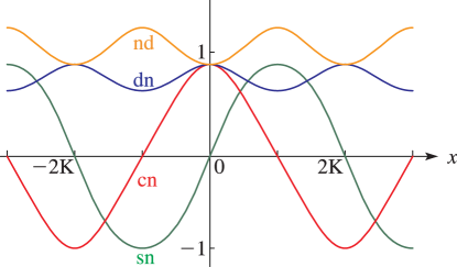
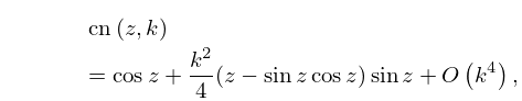
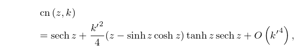
… ►Line graphs of the functions $\mathrm{sn}(x,k)$, $\mathrm{cn}(x,k)$, $\mathrm{dn}(x,k)$, $\mathrm{cd}(x,k)$, $\mathrm{sd}(x,k)$, $\mathrm{nd}(x,k)$, $\mathrm{dc}(x,k)$, $\mathrm{nc}(x,k)$, $\mathrm{sc}(x,k)$, $\mathrm{ns}(x,k)$, $\mathrm{ds}(x,k)$, and $\mathrm{cs}(x,k)$ for representative values of real $x$ and real $k$ illustrating the near trigonometric ($k=0$), and near hyperbolic ($k=1$) limits. … ►

►►

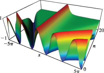
Figure 22.3.2: $k=0.7$, $-3K\le x\le 3K$, $K=1.8456\mathrm{\dots }$. For $\mathrm{cn}(x,k)$ the curve for $k=1/\sqrt{2}=0.70710\mathrm{\dots }$ is a boundary between the curves that have an inflection point in the interval $0\le x\le 2K\left(k\right)$, and its translates, and those that do not; see Walker (1996, p. 146). Magnify

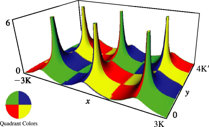
… ► $\mathrm{sn}(x,k)$, $\mathrm{cn}(x,k)$, and $\mathrm{dn}(x,k)$ as functions of real arguments $x$ and $k$. … ►

►

►

Figure 22.3.14: $\mathrm{cn}(x,k)$ for $k=1-{\mathrm{e}}^{-n}$, $n=0$ to 20, $-5\pi \le x\le 5\pi$. Magnify 3D Help

… ►

►

►

Figure 22.3.17: $\mathrm{cn}(x+\mathrm{i}y,k)$ for $k=0.99$, $-3K\le x\le 3K$, $0\le y\le 4K^{\prime }$. … Magnify 3D Help

…