x-difference operators
(0.004 seconds)
11—20 of 86 matching pages
11: About MathML
…
►As a general rule, using the latest available version of your chosen browser, plugins and an updated operating system is helpful.
…
12: 18.1 Notation
…
►
-Differences
►Forward differences: … ►Backward differences: … ►Central differences in imaginary direction: … ►In Koekoek et al. (2010) denotes the operator .13: 31.17 Physical Applications
…
►We use vector notation (respective scalar ) for any one of the three spin operators (respective spin values).
…
►
…
►The operators
and admit separation of variables in , leading to the following factorization of the eigenfunction :
…
14: William P. Reinhardt
…
►Older work on the scattering theory of the atomic Coulomb problem led to the discovery of new classes of orthogonal polynomials relating to the spectral theory of Schrödinger operators, and new uses of old ones: this work was strongly motivated by his original ownership of a 1964 hard copy printing of the original AMS 55 NBS Handbook of Mathematical Functions.
…
15: 1.3 Determinants, Linear Operators, and Spectral Expansions
§1.3 Determinants, Linear Operators, and Spectral Expansions
… ►§1.3(iv) Matrices as Linear Operators
►Linear Operators in Finite Dimensional Vector Spaces
… ►Self-Adjoint Operators on
… ►Real symmetric () and Hermitian () matrices are self-adjoint operators on . …16: 14.30 Spherical and Spheroidal Harmonics
…
►
Parity Operation
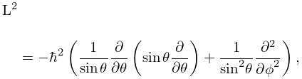
… ►Here, in spherical coordinates, is the squared angular momentum operator: ►
14.30.12
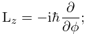
►and is the
component of the angular momentum operator
►
14.30.13
…
17: 1.15 Summability Methods
18: 1.1 Special Notation
19: 10.17 Asymptotic Expansions for Large Argument
…
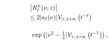
►
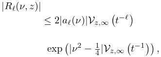
10.17.14
►where denotes the variational operator (2.3.6), and the paths of variation are subject to the condition that changes monotonically.
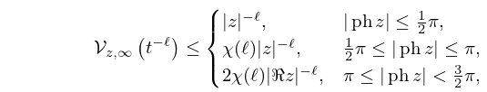
Bounds for are given by
►
10.17.15
…
►The bounds (10.17.15) also apply to in the conjugate sectors.
…
