with respect to integration

SearchAdvancedHelp

(0.006 seconds)

11—20 of 63 matching pages

11: 7.7 Integral Representations

… ►

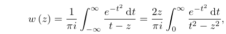
7.7.1 $$\mathrm{erfc}z=\frac{2}{\pi }{\mathrm{e}}^{-z^2}{\int }_0^{\mathrm{\infty }}\frac{{\mathrm{e}}^{-z^2{t}^2}}{t^2+1}dt,$$ $|\mathrm{ph}z|\le \frac{1}{4}\pi$,

ⓘ

Symbols:

$\pi$: the ratio of the circumference of a circle to its diameter, $\mathrm{erfc}z$: complementary error function, $dx$: differential of $x$ , $\mathrm{e}$: base of natural logarithm, $\int$: integral, $\mathrm{ph}$: phase and $z$: complex variable

A&S Ref:

7.4.11 (in different form)

Referenced by:

§7.11, §7.7(i)

Permalink:

http://dlmf.nist.gov/7.7.E1

Encodings:

pMML, png, TeX

See also:

Annotations for §7.7(i), §7.7 and Ch.7

►

7.7.2 $$w\left(z\right)=\frac{1}{\pi \mathrm{i}}{\int }_{-\mathrm{\infty }}^{\mathrm{\infty }}\frac{{\mathrm{e}}^{-t^2}dt}{t-z}=\frac{2z}{\pi \mathrm{i}}{\int }_0^{\mathrm{\infty }}\frac{{\mathrm{e}}^{-t^2}dt}{t^2-z^2},$$ $\mathrm{\Im }z>0$.

ⓘ

Symbols:

$\pi$: the ratio of the circumference of a circle to its diameter, $dx$: differential of $x$ , $w\left(z\right)$: Faddeeva (or Faddeyeva) function, $\mathrm{e}$: base of natural logarithm, $\mathrm{\Im }$: imaginary part, $\mathrm{i}$: imaginary unit, $\int$: integral and $z$: complex variable

A&S Ref:

7.1.4 (in different form)

Referenced by:

§7.19(i), §7.22(i), §7.7(i)

Permalink:

http://dlmf.nist.gov/7.7.E2

Encodings:

pMML, png, TeX

See also:

Annotations for §7.7(i), §7.7 and Ch.7

►

7.7.3 $${\int }_0^{\mathrm{\infty }}{\mathrm{e}}^{-a{t}^2+2\mathrm{i}zt}dt=\frac{1}{2}\sqrt{\frac{\pi }{a}}{\mathrm{e}}^{-z^2/a}+\frac{\mathrm{i}}{\sqrt{a}}F\left(\frac{z}{\sqrt{a}}\right),$$ $\mathrm{\Re }a>0$.

ⓘ

Symbols:

$F\left(z\right)$: Dawson’s integral, $\pi$: the ratio of the circumference of a circle to its diameter, $dx$: differential of $x$ , $\mathrm{e}$: base of natural logarithm, $\mathrm{i}$: imaginary unit, $\int$: integral, $\mathrm{\Re }$: real part and $z$: complex variable

A&S Ref:

7.4.6 7.4.7 (in different notation)

Referenced by:

§7.14(i), §7.7(i)

Permalink:

http://dlmf.nist.gov/7.7.E3

Encodings:

pMML, png, TeX

See also:

Annotations for §7.7(i), §7.7 and Ch.7

… ►

7.7.9 $${\int }_0^x\mathrm{erf}tdt=x\mathrm{erf}x+\frac{1}{\sqrt{\pi }}\left({\mathrm{e}}^{-x^2}-1\right).$$

ⓘ

Symbols:

$\pi$: the ratio of the circumference of a circle to its diameter, $dx$: differential of $x$ , $\mathrm{erf}z$: error function, $\mathrm{e}$: base of natural logarithm, $\int$: integral and $x$: real variable

A&S Ref:

7.4.35 (in different form)

Referenced by:

§7.7(i)

Permalink:

http://dlmf.nist.gov/7.7.E9

Encodings:

pMML, png, TeX

See also:

Annotations for §7.7(i), §7.7 and Ch.7

… ►In (7.7.13) and (7.7.14) the integration paths are straight lines, $\zeta =\frac{1}{16}{\pi }^2{z}^4$, and $c$ is a constant such that in (7.7.13), and in (7.7.14). …

12: 2.8 Differential Equations with a Parameter

… ►dots denoting differentiations with respect to $\xi$. Then … ►The expansions (2.8.11) and (2.8.12) are both uniform and differentiable with respect to $\xi$. … ►The expansions (2.8.15) and (2.8.16) are both uniform and differentiable with respect to $\xi$. … ►The expansions (2.8.25) and (2.8.26) are both uniform and differentiable with respect to $\xi$. …

13: 2.3 Integrals of a Real Variable

… ►

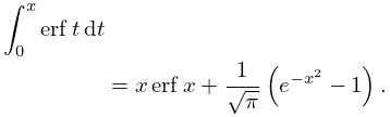
§2.3(i) Integration by Parts

… ►(In other words, differentiation of (2.3.8) with respect to the parameter $\lambda$ (or $\mu$) is legitimate.) … ►derives from the neighborhood of the minimum of $p(t)$ in the integration range. … ►In consequence, the approximation is nonuniform with respect to $\alpha$ and deteriorates severely as $\alpha \to 0$. ►A uniform approximation can be constructed by quadratic change of integration variable: …

14: 4.37 Inverse Hyperbolic Functions

… ►Elsewhere on the integration paths in (4.37.1) and (4.37.2) the branches are determined by continuity. In (4.37.3) the integration path may not intersect $\pm 1$. … ►The principal values (or principal branches) of the inverse $\sinh$, $\cosh$, and $\tanh$ are obtained by introducing cuts in the $z$-plane as indicated in Figure 4.37.1(i)-(iii), and requiring the integration paths in (4.37.1)–(4.37.3) not to cross these cuts. … ►These functions are analytic in the cut plane depicted in Figure 4.37.1(iv), (v), (vi), respectively. … ►are respectively given by …

15: 2.4 Contour Integrals

… ►Then by integration by parts the integral … ►The most successful results are obtained on moving the integration contour as far to the left as possible. … ►

Excluding $t=a$, $\mathrm{\Re }\left({\mathrm{e}}^{\mathrm{i}\theta }p(t)-{\mathrm{e}}^{\mathrm{i}\theta }p(a)\right)$ is positive when $t\in 𝒫$, and is bounded away from zero uniformly with respect to $\theta \in [{\theta }_1,{\theta }_2]$ as $t\to b$ along $𝒫$.

… ►The problem of obtaining an asymptotic approximation to $I(\alpha ,z)$ that is uniform with respect to $\alpha$ in a region containing $\widehat{\alpha }$ is similar to the problem of a coalescing endpoint and saddle point outlined in §2.3(v). ►The change of integration variable is given by …

16: 19.25 Relations to Other Functions

§19.25 Relations to Other Functions

… ►All terms on the right-hand sides are nonnegative when $k^2\le 0$, $0\le k^2\le 1$, or $1\le k^2\le c$, respectively. … ► … ►($F_1$ and $F_D$ are equivalent to the $R$-function of 3 and $n$ variables, respectively, but lack full symmetry.)

17: Bibliography C

… ►

Toward symbolic integration of elliptic integrals. J. Symbolic Comput. 28 (6), pp. 739–753.

ⓘ

Notes:

Code written by J. FitzSimons to generate reduction tables for elliptic integrals symbolically in the Derive computer algebra system is available.

External Links:

ISSN 0747-7171, Document, Code, MathReview (Axel Riese), ZentralBlatt

Referenced by:

§19.29(i), §19.29(ii), §19.29(ii), §19.29(ii), §19.29(ii).

Encodings:

BibTeX

… ►

Elliptic Integrals: Symmetry and Symbolic Integration. In Tricomi’s Ideas and Contemporary Applied Mathematics (Rome/Turin, 1997), Atti dei Convegni Lincei, Vol. 147, pp. 161–181.

ⓘ

External Links:

MathReview (S. L. Kalla), ZentralBlatt

Referenced by:

§19.26(iii), §19.29(i).

Encodings:

BibTeX

… ►

Numerical integration of related Hankel transforms by quadrature and continued fraction expansion. Geophysics 48 (12), pp. 1671–1686.

ⓘ

Notes:

Fortran code.

External Links:

ISSN 0098-3500, Document

Referenced by:

§10.77(ix).

Encodings:

BibTeX

… ►

A method for numerical integration on an automatic copmputer. Numer. Math. 2 (4), pp. 197–205.

ⓘ

External Links:

ISSN 0029-599X, Document, MathReview (A. H. Stroud), ZentralBlatt

Referenced by:

§3.5(iv).

Encodings:

BibTeX

… ►

Derivatives with respect to the degree and order of associated Legendre functions for $|z|>1$ using modified Bessel functions. Integral Transforms Spec. Funct. 21 (7-8), pp. 581–588.

ⓘ

External Links:

ISSN 1065-2469, Document, FullText, MathReview (Dmitriy Karp), ZentralBlatt

Referenced by:

§14.11, §14.11.

Encodings:

BibTeX

…

18: 4.23 Inverse Trigonometric Functions

… ►In (4.23.1) and (4.23.2) the integration paths may not pass through either of the points $t=\pm 1$. The function ${(1-t^2)}^{1/2}$ assumes its principal value when $t\in (-1,1)$; elsewhere on the integration paths the branch is determined by continuity. In (4.23.3) the integration path may not intersect $\pm \mathrm{i}$. … ►The principal values (or principal branches) of the inverse sine, cosine, and tangent are obtained by introducing cuts in the $z$-plane as indicated in Figures 4.23.1(i) and 4.23.1(ii), and requiring the integration paths in (4.23.1)–(4.23.3) not to cross these cuts. … ►are respectively …

19: 28.28 Integrals, Integral Representations, and Integral Equations

… ►

28.28.8 $$\frac{1}{\pi }{\int }_{{ℒ}_j}2\mathrm{i}h\frac{\partial w}{\partial \alpha }{\mathrm{e}}^{2\mathrm{i}hw}{\mathrm{me}}_{\nu }(t,h^2)dt={\mathrm{e}}^{\mathrm{i}\nu \pi /2}{\mathrm{me}}_{\nu }^{\prime }(\alpha ,h^2){\mathrm{M}}_{\nu }^{(j)}(z,h),$$ $j=3,4$,

ⓘ

Symbols:

${\mathrm{me}}_n(z,q)$: Mathieu function, $\pi$: the ratio of the circumference of a circle to its diameter, $dx$: differential of $x$ , $\mathrm{e}$: base of natural logarithm, $\mathrm{i}$: imaginary unit, $\int$: integral, ${\mathrm{M}}_{\nu }^{(j)}(z,h)$: modified Mathieu function, $\frac{\partial f}{\partial x}$: partial derivative of $f$ with respect to $x$ , $\partial x$: partial differential of $x$ , $h$: parameter, $j$: integer, $z$: complex variable, $\nu$: complex parameter, $w(z)$: Mathieu’s equation solution, $\alpha$: parameter and ${ℒ}_j$: integration paths

A&S Ref:

20.7.19 (in slightly different notation)

Permalink:

http://dlmf.nist.gov/28.28.E8

Encodings:

pMML, png, TeX

See also:

Annotations for §28.28(i), §28.28 and Ch.28

…

20: 3.5 Quadrature

… ►

§3.5(iii) Romberg Integration

►Further refinements are achieved by Romberg integration. … ►For these cases the integration path may need to be deformed; see §3.5(ix). … ►A second example is provided in Gil et al. (2001), where the method of contour integration is used to evaluate Scorer functions of complex argument (§9.12). … ►The standard Monte Carlo method samples points uniformly from the integration region to estimate the integral and its error. …