weight functions

SearchAdvancedHelp

(0.004 seconds)

11—20 of 44 matching pages

11: 18.36 Miscellaneous Polynomials

… ►These are OP’s on the interval $(-1,1)$ with respect to an orthogonality measure obtained by adding constant multiples of “Dirac delta weights” at $-1$ and $1$ to the weight function for the Jacobi polynomials. … ►Orthogonality of the the classical OP’s with respect to a positive weight function, as in Table 18.3.1 requires, via Favard’s theorem, $A_n{A}_{n-1}{C}_n>0$ for $n\ge 1$ as per (18.2.9_5). 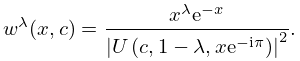… ►implying that, for $n\ge k$, the orthogonality of the $L_n^{(-k)}\left(x\right)$ with respect to the Laguerre weight function $x^{-k}{\mathrm{e}}^{-x}$, $x\in [0,\mathrm{\infty })$. 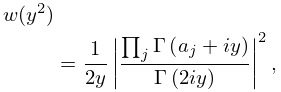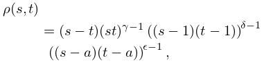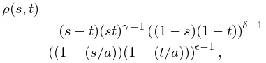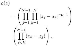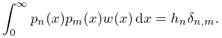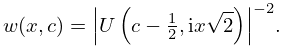… ►Consider the weight function … ►and orthonormal with respect to the weight function …

12: 18.25 Wilson Class: Definitions

… ►

§18.25(ii) Weights and Standardizations: Continuous Cases

►

18.25.2 $${\int }_0^{\mathrm{\infty }}{p}_n(x)p_m(x)w(x)dx=h_n{\delta }_{n,m}.$$

ⓘ

Symbols:

${\delta }_{j,k}$: Kronecker delta, $dx$: differential of $x$ , $\int$: integral, $p_n(x)$: polynomial of degree $n$ , $w(x)$: weight function, $m$: nonnegative integer, $n$: nonnegative integer, $x$: real variable and $h_n$

Permalink:

http://dlmf.nist.gov/18.25.E2

Encodings:

pMML, png, TeX

See also:

Annotations for §18.25(ii), §18.25 and Ch.18

… ►

18.25.4 $$w(y^2)=\frac{1}{2y}{\left|\frac{{\prod }_j\mathrm{\Gamma }\left(a_j+iy\right)}{\mathrm{\Gamma }\left(2iy\right)}\right|}^2,$$

ⓘ

Symbols:

$\mathrm{\Gamma }\left(z\right)$: gamma function, $y$: real variable and $w(x)$: weight function

Permalink:

http://dlmf.nist.gov/18.25.E4

Encodings:

pMML, png, TeX

See also:

Annotations for §18.25(ii), §18.25(ii), §18.25 and Ch.18

… ►

18.25.7 $$w(y^2)=\frac{1}{2y}{\left|\frac{{\prod }_j\mathrm{\Gamma }\left(a_j+iy\right)}{\mathrm{\Gamma }\left(2iy\right)}\right|}^2,$$

ⓘ

Symbols:

$\mathrm{\Gamma }\left(z\right)$: gamma function, $y$: real variable and $w(x)$: weight function

Permalink:

http://dlmf.nist.gov/18.25.E7

Encodings:

pMML, png, TeX

See also:

Annotations for §18.25(ii), §18.25(ii), §18.25 and Ch.18

… ►

18.25.15 $$h_n=\frac{n!(N-n)!{\left(\gamma +\delta +2\right)}_N}{N!{\left(\gamma +1\right)}_n{\left(\delta +1\right)}_{N-n}}.$$

ⓘ

Symbols:

${\left(a\right)}_n$: Pochhammer’s symbol (or shifted factorial), $!$: factorial (as in $n!$), $N$: positive integer, $\delta$: arbitrary small positive constant, $n$: nonnegative integer and $h_n$

Referenced by:

§18.25(iii)

Permalink:

http://dlmf.nist.gov/18.25.E15

Encodings:

pMML, png, TeX

See also:

Annotations for §18.25(iii), §18.25(iii), §18.25 and Ch.18

…

13: 3.11 Approximation Techniques

… ►

§3.11(iii) Minimax Rational Approximations

►Let $f$ be continuous on a closed interval $[a,b]$ and $w$ be a continuous nonvanishing function on $[a,b]$: $w$ is called a weight function. Then the minimax (or best uniform) rational approximation … ► $w(x)$ being a given positive weight function, and again $J\ge n+1$. Then (3.11.29) is replaced by …

14: 31.9 Orthogonality

… ►

31.9.5 $${\int }_{{ℒ}_1}{\int }_{{ℒ}_2}\rho (s,t)w_1(s)w_1(t)w_2(s)w_2(t)dsdt=0,$$ $|n_1-n_2|+|m_1-m_2|\ne 0$,

ⓘ

Symbols:

$dx$: differential of $x$ , $\int$: integral, $m$: nonnegative integer, $n$: nonnegative integer, $\rho (s,t)$: weight function and ${ℒ}_1$, ${ℒ}_2$: integration paths

Permalink:

http://dlmf.nist.gov/31.9.E5

Encodings:

pMML, png, TeX

See also:

Annotations for §31.9(ii), §31.9 and Ch.31

… ►

31.9.6 $$\rho (s,t)=(s-t){(st)}^{\gamma -1}{\left((s-1)(t-1)\right)}^{\delta -1}{\left((s-a)(t-a)\right)}^{ϵ-1},$$

ⓘ

Defines:

$\rho (s,t)$: weight function (locally)

Symbols:

$\gamma$: real or complex parameter, $\delta$: real or complex parameter, $ϵ$: real or complex parameter and $a$: complex parameter

Permalink:

http://dlmf.nist.gov/31.9.E6

Encodings:

pMML, png, TeX

See also:

Annotations for §31.9(ii), §31.9 and Ch.31

…

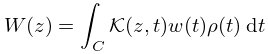
15: 31.10 Integral Equations and Representations

… ►

31.10.1 $$W(z)={\int }_C𝒦(z,t)w(t)\rho (t)dt$$

ⓘ

Defines:

$W(z)$: solution (locally)

Symbols:

$dx$: differential of $x$ , $\int$: integral, $z$: complex variable, $C$: contour, $\rho (t)$: weight function and $𝒦(z,t)$: kernel

Referenced by:

§31.10(i), §31.10(i)

Permalink:

http://dlmf.nist.gov/31.10.E1

Encodings:

pMML, png, TeX

See also:

Annotations for §31.10(i), §31.10 and Ch.31

… ►The weight function is given by ►

31.10.2 $$\rho (t)=t^{\gamma -1}{(t-1)}^{\delta -1}{(t-a)}^{ϵ-1},$$

ⓘ

Defines:

$\rho (t)$: weight function (locally)

Symbols:

$\gamma$: real or complex parameter, $\delta$: real or complex parameter, $ϵ$: real or complex parameter and $a$: complex parameter

Permalink:

http://dlmf.nist.gov/31.10.E2

Encodings:

pMML, png, TeX

See also:

Annotations for §31.10(i), §31.10 and Ch.31

… ►The weight function is ►

31.10.13 $$\rho (s,t)=(s-t){(st)}^{\gamma -1}{\left((1-s)(1-t)\right)}^{\delta -1}{\left((1-(s/a))(1-(t/a))\right)}^{ϵ-1},$$

ⓘ

Defines:

$\rho (s,t)$: weight function (locally)

Symbols:

$\gamma$: real or complex parameter, $\delta$: real or complex parameter, $ϵ$: real or complex parameter and $a$: complex parameter

Permalink:

http://dlmf.nist.gov/31.10.E13

Encodings:

pMML, png, TeX

See also:

Annotations for §31.10(ii), §31.10 and Ch.31

…

16: 31.15 Stieltjes Polynomials

… ►

31.15.11 $${(f,g)}_{\rho }={\int }_{Q}f(z)\overline{g(z)}\rho (z)dz,$$

ⓘ

Symbols:

$\overline{z}$: complex conjugate, $dx$: differential of $x$ , $\int$: integral, $(a,b)$: open interval, $z$: complex variable, $Q$: set and $\rho (z)$: weight function

Permalink:

http://dlmf.nist.gov/31.15.E11

Encodings:

pMML, png, TeX

See also:

Annotations for §31.15(iii), §31.15 and Ch.31

►with weight function ►

31.15.12

ⓘ

Defines:

$\rho (z)$: weight function (locally)

Symbols:

$z$: complex variable, $\gamma$: real or complex parameter, $j$: nonnegative integer, $a$: complex parameter and $N+1$: number of singularities

Permalink:

http://dlmf.nist.gov/31.15.E12

Encodings:

pMML, png, TeX

See also:

Annotations for §31.15(iii), §31.15 and Ch.31

…

17: 18.38 Mathematical Applications

… ►If the nodes in a quadrature formula with a positive weight function are chosen to be the zeros of the $n$th degree OP with the same weight function, and the interval of orthogonality is the same as the integration range, then the weights in the quadrature formula can be chosen in such a way that the formula is exact for all polynomials of degree not exceeding $2n-1$. … ►The basic ideas of Gaussian quadrature, and their extensions to non-classical weight functions, and the computation of the corresponding quadrature abscissas and weights, have led to discrete variable representations, or DVRs, of Sturm–Liouville and other differential operators. …Each of these typically require a particular non-classical weight functions and analysis of the corresponding OP’s. … ►

Non-Classical Weight Functions

…

18: 18.30 Associated OP’s

… ►with weight function ►

18.30.11 $$w^{\lambda }(x,c)=\frac{x^{\lambda }{\mathrm{e}}^{-x}}{{\left|U(c,1-\lambda ,x{\mathrm{e}}^{-\mathrm{i}\pi })\right|}^2}.$$

ⓘ

Symbols:

$U(a,b,z)$: Kummer confluent hypergeometric function, $\pi$: the ratio of the circumference of a circle to its diameter, $\mathrm{e}$: base of natural logarithm, $\mathrm{i}$: imaginary unit, $w(x)$: weight function and $x$: real variable

Permalink:

http://dlmf.nist.gov/18.30.E11

Encodings:

pMML, png, TeX

See also:

Annotations for §18.30(iii), §18.30 and Ch.18

… ►with weight function ►

18.30.15 $$w(x,c)={\left|U(c-\frac{1}{2},\mathrm{i}x\sqrt{2})\right|}^{-2}.$$

ⓘ

Symbols:

$\mathrm{i}$: imaginary unit, $U(a,z)$: parabolic cylinder function, $w(x)$: weight function and $x$: real variable

Permalink:

http://dlmf.nist.gov/18.30.E15

Encodings:

pMML, png, TeX

See also:

Annotations for §18.30(iv), §18.30 and Ch.18

… ►with weight function …

19: Bibliography R

… ►

Erratum to:Relationships between the zeros, weights, and weight functions of orthogonal polynomials: Derivative rule approach to Stieltjes and spectral imaging. Computing in Science and Engineering 23 (4), pp. 91.

ⓘ

External Links:

ISSN 1521-9615, Document, Link

Referenced by:

§18.39(iv), §18.40(ii).

Encodings:

BibTeX

►

Relationships between the zeros, weights, and weight functions of orthogonal polynomials: Derivative rule approach to Stieltjes and spectral imaging. Computing in Science and Engineering 23 (3), pp. 56–64.

ⓘ

External Links:

ISSN 1521-9615, Document, Link

Referenced by:

§18.39(iv), §18.40(ii).

Encodings:

BibTeX

…

20: 18.35 Pollaczek Polynomials

… ►

18.35.6 $$w^{(\lambda )}(\cos \theta ;a,b)={\pi }^{-1}{\mathrm{e}}^{(2\theta -\pi ){\tau }_{a,b}(\theta )}{\left(2\sin \theta \right)}^{2\lambda -1}{\left|\mathrm{\Gamma }\left(\lambda +\mathrm{i}{\tau }_{a,b}(\theta )\right)\right|}^2,$$ .

ⓘ

Symbols:

$\mathrm{\Gamma }\left(z\right)$: gamma function, $\pi$: the ratio of the circumference of a circle to its diameter, $\cos z$: cosine function, $\mathrm{e}$: base of natural logarithm, $\mathrm{i}$: imaginary unit, $\sin z$: sine function, $w(x)$: weight function and ${\tau }_{a,b}(\theta )$

Source:

Ismail (2009, (5.4.13))

Referenced by:

(18.35.5), §18.35(ii), §18.39(iv), §18.39(iv), Erratum (V1.2.0) for Equation (18.35.5)

Permalink:

http://dlmf.nist.gov/18.35.E6

Encodings:

pMML, png, TeX

Modification (effective with 1.2.0):

The constraints in this equation have been moved to (18.35.5) except for .

See also:

Annotations for §18.35(ii), §18.35 and Ch.18

… ►

18.35.6_1

ⓘ

Symbols:

$O\left(x\right)$: order not exceeding, $\pi$: the ratio of the circumference of a circle to its diameter, $\cos z$: cosine function, $\ln z$: principal branch of logarithm function and $w(x)$: weight function

Referenced by:

§18.35(ii), Erratum (V1.2.0) Section 18.35

Permalink:

http://dlmf.nist.gov/18.35.E6_1

Encodings:

pMML, png, TeX

Addition (effective with 1.2.0):

This equation was added.

See also:

Annotations for §18.35(ii), §18.35 and Ch.18

… ►

18.35.6_3 $${\int }_{-1}^1{P}_n^{(\lambda )}(x;a,b)P_m^{(\lambda )}(x;a,b)w^{(\lambda )}(x;a,b)dx+\sum _{\zeta \in D}{P}_n^{(\lambda )}(\zeta ;a,b)P_m^{(\lambda )}(\zeta ;a,b)w_{\zeta }^{(\lambda )}(a,b)=\frac{\mathrm{\Gamma }\left(2\lambda +n\right)}{n!(\lambda +a+n)}{\delta }_{n,m},$$

ⓘ

Symbols:

$\mathrm{\Gamma }\left(z\right)$: gamma function, ${\delta }_{j,k}$: Kronecker delta, $P_n^{(\lambda )}(x;a,b)$: Pollaczek polynomial, $dx$: differential of $x$ , $\in$: element of, $!$: factorial (as in $n!$), $\int$: integral, $(a,b)$: open interval, $w(x)$: weight function, $w_x$: weights, $m$: nonnegative integer, $n$: nonnegative integer and $x$: real variable

Proved:

Ismail (2009, (5.5.18))(proved)

Referenced by:

§18.39(iv)

Permalink:

http://dlmf.nist.gov/18.35.E6_3

Encodings:

pMML, png, TeX

Addition (effective with 1.2.0):

This equation was added.

See also:

Annotations for §18.35(ii), §18.35 and Ch.18

… ►

18.35.6_5 $${\int }_{-1}^1{P}_n^{(\lambda )}(x;a,b,c)P_m^{(\lambda )}(x;a,b,c)w^{(\lambda )}(x;a,b,c)dx=\frac{\mathrm{\Gamma }\left(c+1\right)\mathrm{\Gamma }\left(2\lambda +c+n\right)}{{\left(c+1\right)}_n(\lambda +a+c+n)}{\delta }_{n,m},$$

ⓘ

Symbols:

$\mathrm{\Gamma }\left(z\right)$: gamma function, ${\delta }_{j,k}$: Kronecker delta, ${\left(a\right)}_n$: Pochhammer’s symbol (or shifted factorial), $Q_n^{(\lambda )}(x;a,b,c)$: Pollaczek polynomial, $dx$: differential of $x$ , $\int$: integral, $w(x)$: weight function, $m$: nonnegative integer, $n$: nonnegative integer and $x$: real variable

Proved:

Pollaczek (1950, (3))(proved)

Permalink:

http://dlmf.nist.gov/18.35.E6_5

Encodings:

pMML, png, TeX

Addition (effective with 1.2.0):

This equation was added.

See also:

Annotations for §18.35(ii), §18.35 and Ch.18

… ►

18.35.6_6 $$w^{(\lambda )}(\cos \theta ;a,b,c)=\frac{{\mathrm{e}}^{(2\theta -\pi ){\tau }_{a,b}(\theta )}{\left(2\sin \theta \right)}^{2\lambda -1}{\left|\mathrm{\Gamma }\left(c+\lambda +\mathrm{i}{\tau }_{a,b}(\theta )\right)\right|}^2}{\pi {\left|F(\genfrac{}{}{0pt}{}{1-\lambda +\mathrm{i}{\tau }_{a,b}(\theta ),c}{c+\lambda +\mathrm{i}{\tau }_{a,b}(\theta )};{\mathrm{e}}^{2\mathrm{i}\theta })\right|}^2},$$

ⓘ

Symbols:

$\mathrm{\Gamma }\left(z\right)$: gamma function, $F(a,b;c;z)$ or $F(\genfrac{}{}{0pt}{}{a,b}{c};z)$: $={}_2{}^{}F_1^{}(a,b;c;z)$ Gauss’ hypergeometric function, $\pi$: the ratio of the circumference of a circle to its diameter, $\cos z$: cosine function, $\mathrm{e}$: base of natural logarithm, $\mathrm{i}$: imaginary unit, $\sin z$: sine function, $w(x)$: weight function and ${\tau }_{a,b}(\theta )$

Source:

Pollaczek (1950, (2))

Referenced by:

§18.35(ii), Erratum (V1.2.0) Section 18.35

Permalink:

http://dlmf.nist.gov/18.35.E6_6

Encodings:

pMML, png, TeX

Addition (effective with 1.2.0):

This equation was added.

See also:

Annotations for §18.35(ii), §18.35 and Ch.18

…