ultraspherical polynomials
(0.007 seconds)
11—20 of 32 matching pages
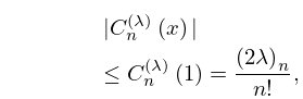
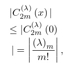
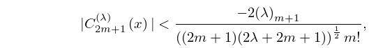
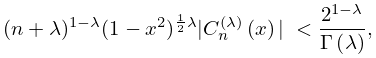
11: 18.14 Inequalities
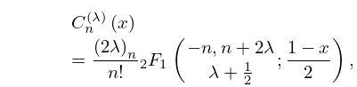
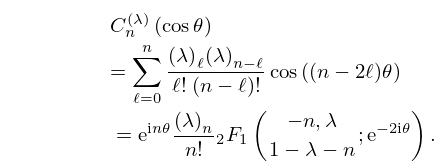
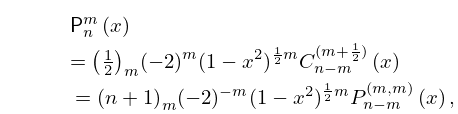
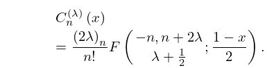
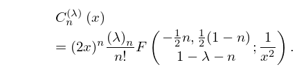
12: 18.5 Explicit Representations
…
►
…
►See (Erdélyi et al., 1953b, §10.9(37)) for a related formula for ultraspherical polynomials.
…
►
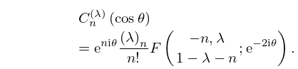
18.5.9
…
►
18.5.11
…
►Similarly in the cases of the ultraspherical polynomials
and the Laguerre polynomials
we assume that , and , unless
stated otherwise.
…
13: 1.10 Functions of a Complex Variable
…
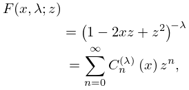
►Ultraspherical polynomials have generating function
►
1.10.28
.
…
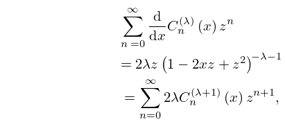
►
1.10.29
►and hence , that is (18.9.19).
The recurrence relation for in §18.9(i) follows from , and the contour integral representation for in §18.10(iii) is just (1.10.27).
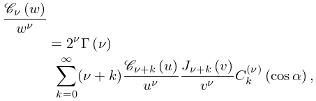
14: 10.23 Sums
15: 18.11 Relations to Other Functions
16: 15.9 Relations to Other Functions
…
►
Gegenbauer (or Ultraspherical)
►
15.9.2
►
15.9.3
►
15.9.4
…
►This is a generalization of Gegenbauer (or ultraspherical) polynomials (§18.3).
…
17: 18.28 Askey–Wilson Class
…
►
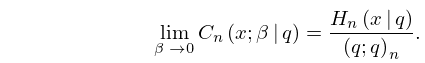
§18.28(v) Continuous -Ultraspherical Polynomials
►
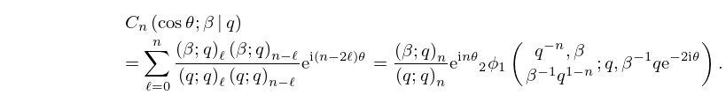
18.28.13
…
►
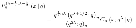
18.28.25
…
►
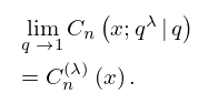
18.28.31
…
►
18.28.32
…
18: 18.35 Pollaczek Polynomials
…
►The type 2 polynomials reduce for to ultraspherical polynomials, see (18.35.8).
…
►
18.35.8
…
►For the ultraspherical polynomials
, the Meixner–Pollaczek polynomials
and the associated Meixner–Pollaczek polynomials
see §§18.3, 18.19 and 18.30(v), respectively.
…
19: 18.15 Asymptotic Approximations
…
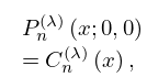
►
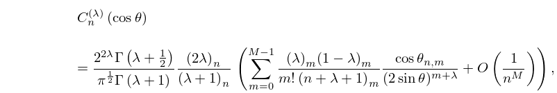
§18.15(ii) Ultraspherical
… ►
18.15.10
…
►Asymptotic expansions for can be obtained from the results given in §18.15(i) by setting and referring to (18.7.1).
…
►For asymptotic approximations of Jacobi, ultraspherical, and Laguerre polynomials in terms of Hermite polynomials, see López and Temme (1999a).
These approximations apply when the parameters are large, namely and (subject to restrictions) in the case of Jacobi polynomials, in the case of ultraspherical polynomials, and in the case of Laguerre polynomials.
…
