…
►Numerical values of
are given in Table
9.7.1 for
to 2D.
…
►In (
9.7.5) and (
9.7.6) the
th error term, that is, the error on
truncating the expansion at
terms, is bounded in magnitude by the first neglected term and has the same sign, provided that the following term is of opposite sign, that is, if
for (
9.7.5) and
for (
9.7.6).
…
►In (
9.7.9)–(
9.7.12) the
th error term in each infinite
series is bounded in magnitude by the first neglected term and has the same sign, provided that the following term in the
series is of opposite sign.
…
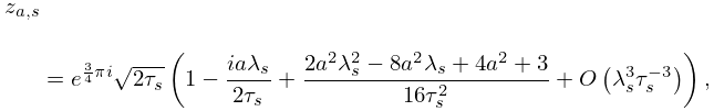
►
,
…
►
…
…
►When
,
, (
25.12.1) becomes
…The cosine
series in (
25.12.7) has the elementary sum
…
►For real or complex
and
the
polylogarithm
is defined by
…
►For each fixed complex
the
series defines an analytic function of
for
.
…
►When
and
, (
25.12.13) becomes (
25.12.4).
…
…
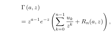
►
8.11.2
.
…
►This reference also contains explicit formulas for the coefficients in terms of Stirling numbers.
…
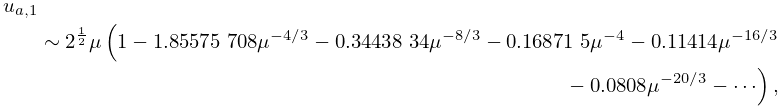
►With
, an asymptotic expansion of
follows from (
8.11.14) and (
8.11.16).
…
►
8.11.14
…
►
8.11.15
…
…
►Walker’s books are
An Introduction to Complex Analysis, published by Hilger in 1974,
The Theory of Fourier Series and Integrals, published by Wiley in 1986,
Elliptic Functions. A Constructive Approach, published by Wiley in 1996, and
Examples and Theorems in Analysis, published by Springer in 2004.
…
►
…
…
►The incomplete integrals
and
can be computed by successive transformations in which two of the three variables converge quadratically to a common value and the integrals reduce to
, accompanied by two quadratically convergent
series in the case of
; compare
Carlson (1965, §§5,6).
…
►If the iteration of (
19.36.6) and (
19.36.12) is stopped when
(
and
being approximated by
and
, and the infinite
series being
truncated), then the relative error in
and
is less than
if we neglect terms of order
.
…
►For computation of Legendre’s integral of the third kind, see
Abramowitz and Stegun (1964, §§17.7 and 17.8, Examples 15, 17, 19, and 20).
…
►For
series expansions of Legendre’s integrals see §
19.5.
Faster convergence of power
series for
and
can be achieved by using (
19.5.1) and (
19.5.2) in the right-hand sides of (
19.8.12).
…
