transformation of variable

SearchAdvancedHelp

(0.004 seconds)

21—30 of 114 matching pages

21: 22.15 Inverse Functions

… ►can be transformed into normal form by elementary change of variables. …

22: 19.36 Methods of Computation

… ►The incomplete integrals $R_F(x,y,z)$ and $R_G(x,y,z)$ can be computed by successive transformations in which two of the three variables converge quadratically to a common value and the integrals reduce to $R_C$, accompanied by two quadratically convergent series in the case of $R_G$; compare Carlson (1965, §§5,6). …

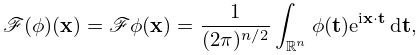
23: 1.9 Calculus of a Complex Variable

… ►

Conformal Transformation

… ► ►

Bilinear Transformation

… ►or its limiting form, and is invariant under bilinear transformations. ►Other names for the bilinear transformation are fractional linear transformation, homographic transformation, and Möbius transformation. …

24: Bille C. Carlson

… ►The main theme of Carlson’s mathematical research has been to expose previously hidden permutation symmetries that can eliminate a set of transformations and thereby replace many formulas by a few. In his paper Lauricella’s hypergeometric function $F_D$ (1963), he defined the $R$-function, a multivariate hypergeometric function that is homogeneous in its variables, each variable being paired with a parameter. If some of the parameters are equal, then the $R$-function is symmetric in the corresponding variables. This symmetry led to the development of symmetric elliptic integrals, which are free from the transformations of modulus and amplitude that complicate the Legendre theory. …Also, the homogeneity of the $R$-function has led to a new type of mean value for several variables, accompanied by various inequalities. …

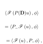
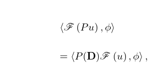
25: 1.16 Distributions

… ►

1.16.29 $$ℱ(\varphi )(𝐱)=ℱ\varphi (𝐱)=\frac{1}{{(2\pi )}^{n/2}}{\int }_{{ℝ}^n}\varphi (𝐭){\mathrm{e}}^{\mathrm{i}𝐱\cdot 𝐭}d𝐭,$$

ⓘ

Defines:

$ℱ(\varphi )$: Fourier transform of a test function (locally)

Symbols:

$\pi$: the ratio of the circumference of a circle to its diameter, $dx$: differential of $x$ , $\mathrm{e}$: base of natural logarithm, $\mathrm{i}$: imaginary unit, $\int$: integral, $ℝ$: real line, $n$: nonnegative integer and $\varphi (x_1,x_2,\mathrm{\dots },x_n)$: test function

Referenced by:

(1.14.1), (1.16.33), (1.16.34), (1.16.35), item (i), item (i)

Permalink:

http://dlmf.nist.gov/1.16.E29

Encodings:

pMML, png, TeX

Notational Change (effective with 1.0.15):

Previously this equation was written as

$$F(𝐱)=F=\frac{1}{{(2\pi )}^{n/2}}{\int }_{{ℝ}^n}\varphi (𝐭){\mathrm{e}}^{\mathrm{i}𝐱\cdot 𝐭}d𝐭.$$

The notation used in §1.14(i) is extended to a test function of several variables.

See also:

Annotations for §1.16(vii), §1.16 and Ch.1

… ►

1.16.33 $$ℱ(P(𝐃)\varphi )(𝐱)=P(-𝐱)ℱ\varphi (𝐱),$$

ⓘ

Symbols:

$\pi$: the ratio of the circumference of a circle to its diameter, $dx$: differential of $x$ , $\mathrm{e}$: base of natural logarithm, $\mathrm{i}$: imaginary unit, $\int$: integral, $ℝ$: real line, $n$: nonnegative integer, $\varphi (x_1,x_2,\mathrm{\dots },x_n)$: test function, $ℱ(\varphi )$: Fourier transform of a test function, $𝐃$: vector differential operator, $P$: polynomial of several variables and $𝐷f$: distributional derivative

Referenced by:

item (iv), §1.16(vii), item (iv)

Permalink:

http://dlmf.nist.gov/1.16.E33

Encodings:

pMML, png, TeX

Notational Change (effective with 1.0.15):

Previously this equation was written as

$$\frac{1}{{(2\pi )}^{n/2}}{\int }_{{ℝ}^n}(P(𝐷)\varphi )(𝐭){\mathrm{e}}^{\mathrm{i}𝐱\cdot 𝐭}d𝐭=P(-𝐱)F(𝐱).$$

It has been rewritten using the notation of (1.16.29) and (1.16.32).

See also:

Annotations for §1.16(vii), §1.16 and Ch.1

… ►

1.16.34 $$ℱ(P\varphi )(𝐱)=P(𝐃)ℱ\varphi (𝐱).$$

ⓘ

Symbols:

$\pi$: the ratio of the circumference of a circle to its diameter, $dx$: differential of $x$ , $\mathrm{e}$: base of natural logarithm, $\mathrm{i}$: imaginary unit, $\int$: integral, $ℝ$: real line, $n$: nonnegative integer, $\varphi (x_1,x_2,\mathrm{\dots },x_n)$: test function, $ℱ(\varphi )$: Fourier transform of a test function, $𝐃$: vector differential operator, $P$: polynomial of several variables and $𝐷f$: distributional derivative

Referenced by:

item (iv), §1.16(vii), item (iv)

Permalink:

http://dlmf.nist.gov/1.16.E34

Encodings:

pMML, png, TeX

Notational Change (effective with 1.0.15):

Previously this equation was written as

$$\frac{1}{{(2\pi )}^{n/2}}{\int }_{{ℝ}^n}P(𝐭)\varphi (𝐭){\mathrm{e}}^{\mathrm{i}𝐱\cdot 𝐭}d𝐭=P(𝐷)F(𝐱).$$

It has been rewritten using the notation of (1.16.29) and (1.16.32).

See also:

Annotations for §1.16(vii), §1.16 and Ch.1

… ►

1.16.36 $$⟨ℱ\left(P(𝐃)u\right),\varphi ⟩=⟨P_{-}ℱ\left(u\right),\varphi ⟩=⟨ℱ\left(u\right),P_{-}\varphi ⟩,$$

ⓘ

Symbols:

$⟨\mathrm{\Lambda },\varphi ⟩$: action of distribution on test function, $ℱ\left(u\right)$: Fourier transform of a tempered distribution, $\varphi (x_1,x_2,\mathrm{\dots },x_n)$: test function, $𝐃$: vector differential operator, $P$: polynomial of several variables and $𝐷f$: distributional derivative

Referenced by:

item (iv), §1.16(vii), §1.16(viii), item (iv)

Permalink:

http://dlmf.nist.gov/1.16.E36

Encodings:

pMML, png, TeX

Notational Change (effective with 1.0.15):

Previously this equation was written as

$$ℱ(P(𝐷)u)=P(-𝐱)ℱ(u).$$

It has been rewritten using the notation of (1.16.32) and (1.16.35).

See also:

Annotations for §1.16(vii), §1.16 and Ch.1

►

1.16.37 $$⟨ℱ\left(Pu\right),\varphi ⟩=⟨P(𝐃)ℱ\left(u\right),\varphi ⟩,$$

ⓘ

Symbols:

$⟨\mathrm{\Lambda },\varphi ⟩$: action of distribution on test function, $ℱ\left(u\right)$: Fourier transform of a tempered distribution, $\varphi (x_1,x_2,\mathrm{\dots },x_n)$: test function, $𝐃$: vector differential operator, $P$: polynomial of several variables and $𝐷f$: distributional derivative

Referenced by:

item (iv), §1.16(vii), item (iv)

Permalink:

http://dlmf.nist.gov/1.16.E37

Encodings:

pMML, png, TeX

Notational Change (effective with 1.0.15):

Previously this equation was written as

$$ℱ(Pu)=P(𝐷)ℱ(u).$$

It has been rewritten using the notation of (1.16.32) and (1.16.35).

See also:

Annotations for §1.16(vii), §1.16 and Ch.1

…

26: 28.2 Definitions and Basic Properties

… ►With $\zeta ={\sin }^{2}z$ we obtain the algebraic form of Mathieu’s equation ►

28.2.2 $$\zeta (1-\zeta )w^{\prime \prime }+\frac{1}{2}(1-2\zeta )w^{\prime }+\frac{1}{4}(a-2q(1-2\zeta ))w=0.$$

ⓘ

Symbols:

$q=h^2$: parameter, $a$: parameter, $w(z)$: Mathieu’s equation solution and $\zeta$: change of variable

Permalink:

http://dlmf.nist.gov/28.2.E2

Encodings:

pMML, png, TeX

See also:

Annotations for §28.2(i), §28.2 and Ch.28

… ►Furthermore, a solution $w$ with given initial constant values of $w$ and $w^{\prime }$ at a point $z_0$ is an entire function of the three variables $z$, $a$, and $q$. ►The following three transformations … ►

$z\to z\pm \frac{1}{2}\pi ,q\to -q;$

…

27: 10.43 Integrals

… ►

10.43.30 $$f(y)=\frac{2y}{{\pi }^2}\sinh \left(\pi y\right){\int }_0^{\mathrm{\infty }}\frac{g(x)}{x}{K}_{\mathrm{i}y}\left(x\right)dx.$$

ⓘ

Defines:

$f(x)$: Kontorovich–Lebedev transform of $g(x)$ (locally)

Symbols:

$\pi$: the ratio of the circumference of a circle to its diameter, $dx$: differential of $x$ , $\sinh z$: hyperbolic sine function, $\mathrm{i}$: imaginary unit, $\int$: integral, $K_{\nu }\left(z\right)$: modified Bessel function of the second kind, $x$: real variable, $y$: real variable and $g(x)$: function

Referenced by:

§10.43(v)

Permalink:

http://dlmf.nist.gov/10.43.E30

Encodings:

pMML, png, TeX

See also:

Annotations for §10.43(v), §10.43 and Ch.10

… ►

10.43.31 $$g(x)={\int }_0^{\mathrm{\infty }}f(y)K_{\mathrm{i}y}\left(x\right)dy,$$

ⓘ

Symbols:

$dx$: differential of $x$ , $\mathrm{i}$: imaginary unit, $\int$: integral, $K_{\nu }\left(z\right)$: modified Bessel function of the second kind, $x$: real variable, $y$: real variable, $g(x)$: function and $f(x)$: Kontorovich–Lebedev transform of $g(x)$

Referenced by:

§10.43(v)

Permalink:

http://dlmf.nist.gov/10.43.E31

Encodings:

pMML, png, TeX

See also:

Annotations for §10.43(v), §10.43 and Ch.10

…

28: 2.8 Differential Equations with a Parameter

… ►The transformation is now specialized in such a way that: (a) $\xi$ and $z$ are analytic functions of each other at the transition point (if any); (b) the approximating differential equation obtained by neglecting $\psi (\xi )$ (or part of $\psi (\xi )$) has solutions that are functions of a single variable. …

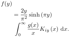
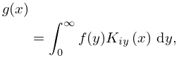
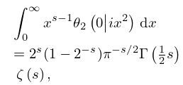
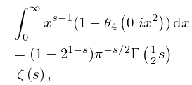
29: 20.10 Integrals

… ►

§20.10(i) Mellin Transforms with respect to the Lattice Parameter

►

20.10.1 $${\int }_0^{\mathrm{\infty }}{x}^{s-1}{\theta }_2\left(0\right|\mathrm{i}{x}^2)dx=2^s(1-2^{-s}){\pi }^{-s/2}\mathrm{\Gamma }\left(\frac{1}{2}s\right)\zeta \left(s\right),$$ $\mathrm{\Re }s>1$,

ⓘ

Symbols:

$\mathrm{\Gamma }\left(z\right)$: gamma function, ${\theta }_j\left(z\right|\tau )$: theta function, $\zeta \left(s\right)$: Riemann zeta function, $\pi$: the ratio of the circumference of a circle to its diameter, $dx$: differential of $x$ , $\mathrm{i}$: imaginary unit, $\int$: integral and $\mathrm{\Re }$: real part

Keywords:

Mellin transform

Referenced by:

§20.10(i), Erratum (V1.1.5) for §20.10(i)

Permalink:

http://dlmf.nist.gov/20.10.E1

Encodings:

pMML, png, TeX

Modification (effective with 1.1.5):

Originally the constraint was $\mathrm{\Re }s>2$. This can be relaxed to $\mathrm{\Re }s>1$ because ${\theta }_2\left(0\right|\mathrm{i}{x}^2)=x^{-1}{\theta }_4\left(0\right|\mathrm{i}{x}^{-2})\sim x^{-1}$ as $x\to 0+$, which follows from (20.7.31) and (20.4.5).

See also:

Annotations for §20.10(i), §20.10 and Ch.20

►

20.10.2 $${\int }_0^{\mathrm{\infty }}{x}^{s-1}({\theta }_3\left(0\right|\mathrm{i}{x}^2)-1)dx={\pi }^{-s/2}\mathrm{\Gamma }\left(\frac{1}{2}s\right)\zeta \left(s\right),$$ $\mathrm{\Re }s>1$,

ⓘ

Symbols:

$\mathrm{\Gamma }\left(z\right)$: gamma function, ${\theta }_j\left(z\right|\tau )$: theta function, $\zeta \left(s\right)$: Riemann zeta function, $\pi$: the ratio of the circumference of a circle to its diameter, $dx$: differential of $x$ , $\mathrm{i}$: imaginary unit, $\int$: integral and $\mathrm{\Re }$: real part

Keywords:

Mellin transform

Referenced by:

§20.10(i), Erratum (V1.1.5) for §20.10(i)

Permalink:

http://dlmf.nist.gov/20.10.E2

Encodings:

pMML, png, TeX

Modification (effective with 1.1.5):

Originally the constraint was $\mathrm{\Re }s>2$. This can be relaxed to $\mathrm{\Re }s>1$ because ${\theta }_3\left(0\right|\mathrm{i}{x}^2)=x^{-1}{\theta }_3\left(0\right|\mathrm{i}{x}^{-2})\sim x^{-1}$ as $x\to 0+$, which follows from (20.7.32) and (20.4.4).

See also:

Annotations for §20.10(i), §20.10 and Ch.20

►

20.10.3 $${\int }_0^{\mathrm{\infty }}{x}^{s-1}(1-{\theta }_4\left(0\right|\mathrm{i}{x}^2))dx=(1-2^{1-s}){\pi }^{-s/2}\mathrm{\Gamma }\left(\frac{1}{2}s\right)\zeta \left(s\right),$$ $\mathrm{\Re }s>0$.

ⓘ

Symbols:

$\mathrm{\Gamma }\left(z\right)$: gamma function, ${\theta }_j\left(z\right|\tau )$: theta function, $\zeta \left(s\right)$: Riemann zeta function, $\pi$: the ratio of the circumference of a circle to its diameter, $dx$: differential of $x$ , $\mathrm{i}$: imaginary unit, $\int$: integral and $\mathrm{\Re }$: real part

Keywords:

Mellin transform

Referenced by:

§20.10(i), Erratum (V1.1.5) for §20.10(i)

Permalink:

http://dlmf.nist.gov/20.10.E3

Encodings:

pMML, png, TeX

Modification (effective with 1.1.5):

Originally the constraint was $\mathrm{\Re }s>2$. This can be relaxed to $\mathrm{\Re }s>0$ because $1-{\theta }_4\left(0\right|\mathrm{i}{x}^2)=1-x^{-1}{\theta }_2\left(0\right|\mathrm{i}{x}^{-2})\sim 1$ as $x\to 0+$, which follows from (20.7.33) and (20.4.3).

See also:

Annotations for §20.10(i), §20.10 and Ch.20

… ►

§20.10(ii) Laplace Transforms with respect to the Lattice Parameter

…

30: 1.12 Continued Fractions

… ►

Fractional Transformations

… ►

1.12.20 $$C_n(w)=b_0+\frac{a_1}{b_1+}\frac{a_2}{b_2+}\mathrm{\cdots }\frac{a_n}{b_n+w}.$$

ⓘ

Symbols:

$w$: variable, $n$: nonnegative integer and $C_n(w)$: continued fraction

Referenced by:

§1.12(ii)

Permalink:

http://dlmf.nist.gov/1.12.E20

Encodings:

pMML, png, TeX

See also:

Annotations for §1.12(ii), §1.12(ii), §1.12 and Ch.1

…