symmetric case
(0.002 seconds)
11—20 of 40 matching pages
11: 19.36 Methods of Computation
…
►Complete cases of Legendre’s integrals and symmetric integrals can be computed with quadratic convergence by the AGM method (including Bartky transformations), using the equations in §19.8(i) and §19.22(ii), respectively.
…
12: 19.26 Addition Theorems
§19.26 Addition Theorems
… ►§19.26(ii) Case
… ►§19.26(iii) Duplication Formulas
… ►
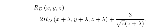
19.26.20
►
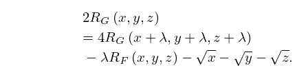
19.26.21
…
13: 3.2 Linear Algebra
…
►Then in all cases.
…
►The Euclidean norm is the case
.
…
►When is a symmetric matrix, the left and right eigenvectors coincide, yielding , and the calculation of its eigenvalues is a well-conditioned problem.
►
§3.2(vi) Lanczos Tridiagonalization of a Symmetric Matrix
►Let be an symmetric matrix. …14: 1.3 Determinants, Linear Operators, and Spectral Expansions
…
►In the case of a real matrix and in the complex case
.
►Real symmetric () and Hermitian () matrices are self-adjoint operators on .
…
►For Hermitian matrices is unitary, and for real symmetric matrices is an orthogonal transformation.
…
15: 19.17 Graphics
§19.17 Graphics
►See Figures 19.17.1–19.17.8 for symmetric elliptic integrals with real arguments. … ►For , , and , which are symmetric in , we may further assume that is the largest of if the variables are real, then choose , and consider only and . The cases or correspond to the complete integrals. The case corresponds to elementary functions. …16: 19.29 Reduction of General Elliptic Integrals
…
►The advantages of symmetric integrals for tables of integrals and symbolic integration are illustrated by (19.29.4) and its cubic case, which replace the formulas in Gradshteyn and Ryzhik (2000, 3.147, 3.131, 3.152) after taking as the variable of integration in 3.
…
17: 19.22 Quadratic Transformations
…
►
Bartky’s Transformation
… ►§19.22(ii) Gauss’s Arithmetic-Geometric Mean (AGM)
… ►Descending Gauss transformations include, as special cases, transformations of complete integrals into complete integrals; ascending Landen transformations do not. … ►18: 19.7 Connection Formulas
…
►
§19.7(iii) Change of Parameter of
… ►If and are real, then both integrals are circular cases or both are hyperbolic cases (see §19.2(ii)). ►The first of the three relations maps each circular region onto itself and each hyperbolic region onto the other; in particular, it gives the Cauchy principal value of when (see (19.6.5) for the complete case). …19: 19.33 Triaxial Ellipsoids
…
►
19.33.1
…
►
§19.33(ii) Potential of a Charged Conducting Ellipsoid
… ►
19.33.5
…
►
19.33.6
►A conducting elliptic disk is included as the case
.
…
20: 18.38 Mathematical Applications
…
►
