strict shifted
(0.002 seconds)
1—10 of 155 matching pages
1: 26.12 Plane Partitions
…
►
26.12.17
►A strict shifted plane partition is an arrangement of the parts in a partition so that each row is indented one space from the previous row and there is weak decrease across rows and strict decrease down columns.
…
►A descending plane partition is a strict shifted plane partition in which the number of parts in each row is strictly less than the largest part in that row and is greater than or equal to the largest part in the next row.
The example of a strict shifted plane partition also satisfies the conditions of a descending plane partition.
…
2: 33.25 Approximations
§33.25 Approximations
►Cody and Hillstrom (1970) provides rational approximations of the phase shift (see (33.2.10)) for the ranges , , and . …3: 26.10 Integer Partitions: Other Restrictions
…
►Note that , with strict inequality for .
It is known that for , , with strict inequality for sufficiently large, provided that , or ; see Yee (2004).
…
4: Possible Errors in DLMF
…
►One source of confusion, rather than actual errors, are some new functions which differ from those in Abramowitz and Stegun (1964) by scaling, shifts or constraints on the domain; see the Info box (click or hover over the ![[Uncaptioned image]](../help/g3.png) icon) for links to defining formula.
…
icon) for links to defining formula.
…
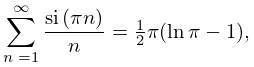
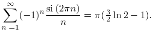
5: 6.15 Sums
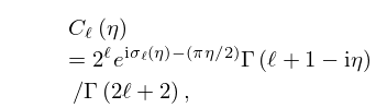
6: 33.13 Complex Variable and Parameters
…
►The quantities , , and , given by (33.2.6), (33.2.10), and (33.4.1), respectively, must be defined consistently so that
►
33.13.1
…
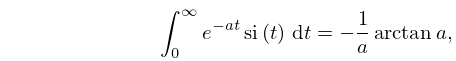
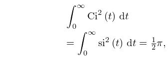
7: 6.14 Integrals
8: 18.3 Definitions
…
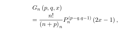
►
…
9: 35.4 Partitions and Zonal Polynomials
…
►Also, denotes , the weight of ; denotes the number of nonzero ; denotes the vector .
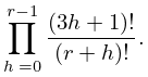
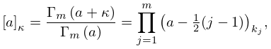
►The partitional shifted factorial is given by
►
35.4.1
…
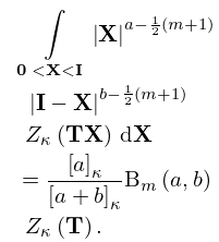
►
35.4.2
…
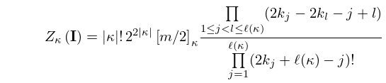
►
35.4.9
