stable

SearchAdvancedHelp

(0.001 seconds)

1—10 of 20 matching pages

1: 28.17 Stability as $x\to \pm \mathrm{\infty }$

§28.17 Stability as $x\to \pm \mathrm{\infty }$

►If all solutions of (28.2.1) are bounded when $x\to \pm \mathrm{\infty }$ along the real axis, then the corresponding pair of parameters $(a,q)$ is called stable. … ►For example, positive real values of $a$ with $q=0$ comprise stable pairs, as do values of $a$ and $q$ that correspond to real, but noninteger, values of $\nu$. … ►For real $a$ and $q$ $(\ne 0)$ the stable regions are the open regions indicated in color in Figure 28.17.1. … ►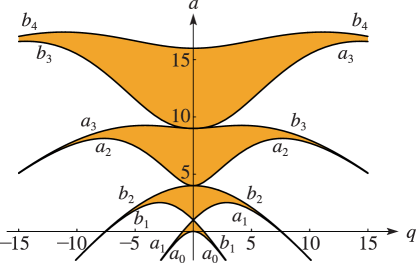

►►

Figure 28.17.1: Stability chart for eigenvalues of Mathieu’s equation (28.2.1). Magnify

2: 14.32 Methods of Computation

… ►In particular, for small or moderate values of the parameters $\mu$ and $\nu$ the power-series expansions of the various hypergeometric function representations given in §§14.3(i)–14.3(iii), 14.19(ii), and 14.20(i) can be selected in such a way that convergence is stable, and reasonably rapid, especially when the argument of the functions is real. In other cases recurrence relations (§14.10) provide a powerful method when applied in a stable direction (§3.6); see Olver and Smith (1983) and Gautschi (1967). …

3: 29.9 Stability

… ►The Lamé equation (29.2.1) with specified values of $k,h,\nu$ is called stable if all of its solutions are bounded on $ℝ$; otherwise the equation is called unstable. …

4: 33.23 Methods of Computation

… ►When numerical values of the Coulomb functions are available for some radii, their values for other radii may be obtained by direct numerical integration of equations (33.2.1) or (33.14.1), provided that the integration is carried out in a stable direction (§3.7). … ►In a similar manner to §33.23(iii) the recurrence relations of §§33.4 or 33.17 can be used for a range of values of the integer $\mathrm{\ell }$, provided that the recurrence is carried out in a stable direction (§3.6). …

5: 1.11 Zeros of Polynomials

§1.11 Zeros of Polynomials

… ►

§1.11(v) Stable Polynomials

… ►with real coefficients, is called stable if the real parts of all the zeros are strictly negative. ►

Hurwitz Criterion

… ►Then $f(z)$, with $a_n\ne 0$, is stable iff $a_0\ne 0$; $D_{2k}>0$, $k=1,\mathrm{\dots },\lfloor \frac{1}{2}n\rfloor$; $\mathrm{sign}{D}_{2k+1}=\mathrm{sign}{a}_0$, $k=0,1,\mathrm{\dots },\lfloor \frac{1}{2}n-\frac{1}{2}\rfloor$.

6: 36.14 Other Physical Applications

… ►These are the structurally stable focal singularities (envelopes) of families of rays, on which the intensities of the geometrical (ray) theory diverge. …

7: 8.25 Methods of Computation

… ►Stable recursive schemes for the computation of $E_p\left(x\right)$ are described in Miller (1960) for $x>0$ and integer $p$. …

8: 9.17 Methods of Computation

… ►In the case of the Scorer functions, integration of the differential equation (9.12.1) is more difficult than (9.2.1), because in some regions stable directions of integration do not exist. …

9: 11.13 Methods of Computation

… ►Then from the limiting forms for small argument (§§11.2(i), 10.7(i), 10.30(i)), limiting forms for large argument (§§11.6(i), 10.7(ii), 10.30(ii)), and the connection formulas (11.2.5) and (11.2.6), it is seen that ${𝐇}_{\nu }\left(x\right)$ and ${𝐋}_{\nu }\left(x\right)$ can be computed in a stable manner by integrating forwards, that is, from the origin toward infinity. …

10: 28.33 Physical Applications

… ►Hence from §28.17 the corresponding Mathieu equation is stable or unstable according as $(q,a)$ is in the intersection of $ℒ$ with the colored or the uncolored open regions depicted in Figure 28.17.1. In particular, the equation is stable for all sufficiently large values of $\omega$. …