spherical (or spherical polar)
(0.001 seconds)
11—20 of 84 matching pages
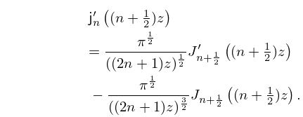
11: 10.51 Recurrence Relations and Derivatives
12: 10.57 Uniform Asymptotic Expansions for Large Order
§10.57 Uniform Asymptotic Expansions for Large Order
►Asymptotic expansions for , , , , , and as that are uniform with respect to can be obtained from the results given in §§10.20 and 10.41 by use of the definitions (10.47.3)–(10.47.7) and (10.47.9). Subsequently, for the connection formula (10.47.11) is available. ►For the corresponding expansion for use ►
10.57.1
…
13: 10.58 Zeros
§10.58 Zeros
►For the th positive zeros of , , , and are denoted by , , , and , respectively, except that for we count as the first zero of . … ►14: 10.1 Special Notation
…
►The main functions treated in this chapter are the Bessel functions , ; Hankel functions , ; modified Bessel functions , ; spherical Bessel functions , , , ; modified spherical Bessel functions , , ; Kelvin functions , , , .
For the spherical Bessel functions and modified spherical Bessel functions the order is a nonnegative integer.
…
►Abramowitz and Stegun (1964): , , , , for , , , , respectively, when .
…
►For older notations see British Association for the Advancement of Science (1937, pp. xix–xx) and Watson (1944, Chapters 1–3).
15: 10.54 Integral Representations
§10.54 Integral Representations
… ►
10.54.2
►
10.54.3
…
►
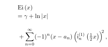
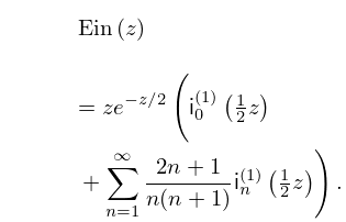
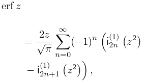
16: 6.10 Other Series Expansions
…
►
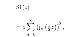
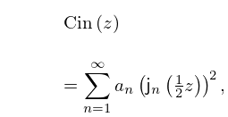
§6.10(ii) Expansions in Series of Spherical Bessel Functions
… ►
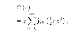
6.10.4
►
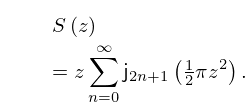
6.10.5
►
6.10.6
,
…
►
6.10.8
…
17: 10.73 Physical Applications
…
►
…
►
§10.73(ii) Spherical Bessel Functions
►The functions , , , and arise in the solution (again by separation of variables) of the Helmholtz equation in spherical coordinates (§1.5(ii)): …With the spherical harmonic defined as in §14.30(i), the solutions are of the form with , , , or , depending on the boundary conditions. Accordingly, the spherical Bessel functions appear in all problems in three dimensions with spherical symmetry involving the scattering of electromagnetic radiation. …18: 10.59 Integrals
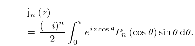
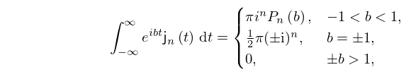
§10.59 Integrals
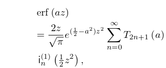
►
10.59.1
►where is the Legendre polynomial (§18.3).
►For an integral representation of the Dirac delta in terms of a product of spherical Bessel functions of the first kind see §1.17(ii), and for a generalization see Maximon (1991).
…
