spherical%20polar%20coordinates
(0.003 seconds)
1—10 of 195 matching pages
1: 14.30 Spherical and Spheroidal Harmonics
…
►
§14.30(i) Definitions
… ► … ►As an example, Laplace’s equation in spherical coordinates (§1.5(ii)): … ►Here, in spherical coordinates, is the squared angular momentum operator: … ►2: 10.73 Physical Applications
…
►See Krivoshlykov (1994, Chapter 2, §2.2.10; Chapter 5, §5.2.2), Kapany and Burke (1972, Chapters 4–6; Chapter 7, §A.1), and Slater (1942, Chapter 4, §§20, 25).
…
►
…
►
§10.73(ii) Spherical Bessel Functions
►The functions , , , and arise in the solution (again by separation of variables) of the Helmholtz equation in spherical coordinates (§1.5(ii)): …Accordingly, the spherical Bessel functions appear in all problems in three dimensions with spherical symmetry involving the scattering of electromagnetic radiation. …3: 10.75 Tables
…
►
•
►
•
►
•
…
§10.75(ix) Spherical Bessel Functions, Modified Spherical Bessel Functions, and their Derivatives
►Zhang and Jin (1996, pp. 296–305) tabulates , , , , , , , , , 50, 100, , 5, 10, 25, 50, 100, 8S; , , , (Riccati–Bessel functions and their derivatives), , 50, 100, , 5, 10, 25, 50, 100, 8S; real and imaginary parts of , , , , , , , , , 20(10)50, 100, , , 8S. (For the notation replace by , , , , respectively.)
§10.75(x) Zeros and Associated Values of Derivatives of Spherical Bessel Functions
… ►Olver (1960) tabulates , , , , , , 8D. Also included are tables of the coefficients in the uniform asymptotic expansions of these zeros and associated values as .
4: 20 Theta Functions
Chapter 20 Theta Functions
…5: 10.55 Continued Fractions
§10.55 Continued Fractions
►For continued fractions for and see Cuyt et al. (2008, pp. 350, 353, 362, 363, 367–369).6: 18.39 Applications in the Physical Sciences
…
►Now use spherical coordinates (1.5.16) with instead of , and assume the potential to be radial.
…By (1.5.17) the first term in (18.39.21), which is the quantum kinetic energy operator , can be written in spherical coordinates
as
…
…
►
a) Spherical Radial Coulomb Wave Functions Expressed in terms of Laguerre OP’s
… ►c) Spherical Radial Coulomb Wave Functions
…7: 10.48 Graphs
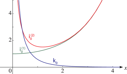
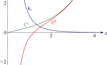
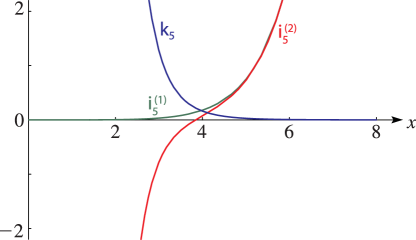
§10.48 Graphs
… ► ►
►
 ►
►
 ►
►
8: 1.5 Calculus of Two or More Variables
…
►
